Math basic of 3D Reconstruction

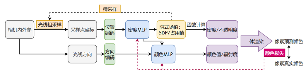
Framework

相机内外惨：连接像素坐标系与空间坐标系之间的计算
隐式implicit场：通过一个隐式表示的函数表示物体/场景，使用MLP来学习空间的隐式函数
- 密度场，表示该空间点的密度
- SDF $sdf=F(x,y,z)=0$，表示该空间点离物体表面的最近距离
编码：由于直接使用输入坐标xyz，网络无法很好地学习低频特征，需要将其进行高频编码
空间点采样：逆变换采样CDF
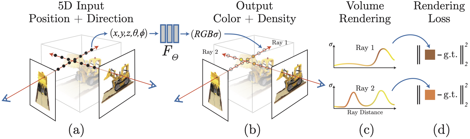
体渲染：将沿着光线空间采样点的颜色和密度积分为像素颜色

体渲染函数

Ray: $\mathbf{r} = \mathbf{o} +t\mathbf{d}$

密度场:（NeRF）
$\mathrm{C}(r)=\int_{\mathrm{t}_{\mathrm{n}}}^{\mathrm{t}_{\mathrm{f}}} \mathrm{T}(\mathrm{t}) \sigma(\mathrm{r}(\mathrm{t})) \mathrm{c}(\mathrm{r}(\mathrm{t}), \mathrm{d}) \mathrm{dt}$

$\mathrm{T}(\mathrm{t})=\exp \left(-\int_{\mathrm{t}_{\mathrm{n}}}^{\mathrm{t}} \sigma(\mathrm{r}(\mathrm{s})) \mathrm{ds}\right)$
累计透射率$T(t)$可以保证离相机位置近的地方有更大的权重(一条光线前面的点遮挡后面的点)
离散化：$\hat{C}(\mathbf{r})=\sum_{i=1}^{N} T_{i}\alpha_{i}\mathbf{c}_{i}=\sum_{i=1}^{N} T_{i}\left(1-\exp \left(-\sigma_{i} \delta_{i}\right)\right) \mathbf{c}_{i}$
$T_{i}=\exp \left(-\sum_{j=1}^{i-1} \sigma_{j} \delta_{j}\right)=\prod_{j=1}^{i-1}(1-\alpha_j)$

符号距离函数SDF：(NeuS)
$C(\mathbf{o},\mathbf{v})=\int_{0}^{+\infty}w(t)c(\mathbf{p}(t),\mathbf{d})\mathrm{d}t$

$\omega(t)=T(t)\rho(t),\text{where}T(t)=\exp\left(-\int_0^t\rho(u)\mathrm{d}u\right)$
$\rho(t)=\max\left(\frac{-\frac{\mathrm{d}\Phi_s}{\mathrm{d}t}(f(\mathbf{p}(t)))}{\Phi_s(f(\mathbf{p}(t)))},0\right)$
离散化：$\hat{C}=\sum_{i=1}^n T_i\alpha_i c_i$
$T_i=\prod_{j=1}^{i-1}(1-\alpha_j)$
$\alpha_i=\max\left(\frac{\Phi_s(f(\mathbf{p}(t_i))))-\Phi_s(f(\mathbf{p}(t_{i+1})))}{\Phi_s(f(\mathbf{p}(t_i)))},0\right)$

坐标变换

【相机标定】相机标定原理 - welcome to x-jeff blog 相机内外参+径切向畸变

矩阵的QR分解

QR分解可以将任何实数方阵分解成一个正交矩阵Q与一个上三角矩阵R的积

$A=QR$

# This function is borrowed from IDR: https://github.com/lioryariv/idr
def load_K_Rt_from_P(P=None):
    # P : 3x4
    out = cv.decomposeProjectionMatrix(P) # 基于QR分解
    K = out[0] # 3x3
    R = out[1] # 3x3
    t = out[2] # 3x1

    K = K / K[2, 2]
    intrinsics = np.eye(4)
    intrinsics[:3, :3] = K # intrinsics: 4x4 为相机内参矩阵

    pose = np.eye(4, dtype=np.float32)
    pose[:3, :3] = R.transpose()
    pose[:3, 3] = (t[:3] / t[3])[:, 0] # pose: 4x4 为相机外参矩阵

    return intrinsics, pose
  
P = (world_mat @ scale_mat)[:3, :4] # ws2p矩阵
intrinsics, pose = load_K_Rt_from_P(P) # 将 ws2p矩阵分解为 c2p和c2ws矩阵

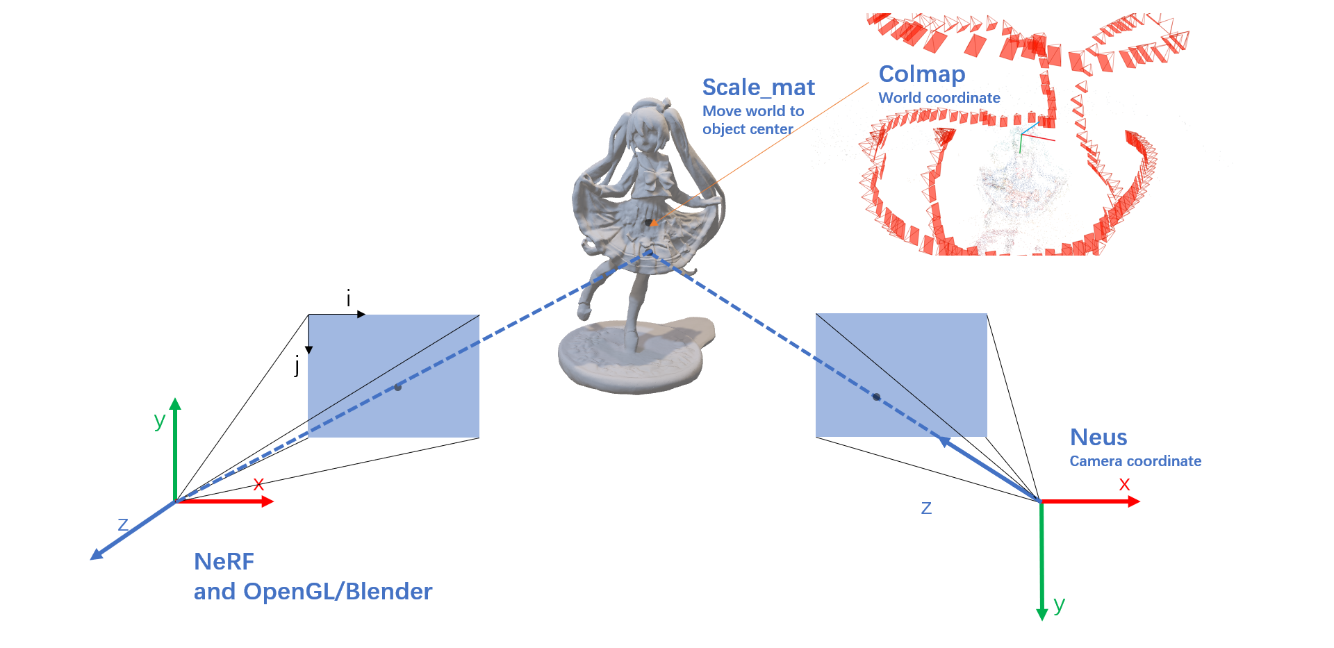
world_mat 为 w2p矩阵
scale_mat 为 ws2w矩阵，其中ws是单位box坐标系，坐标原点在box中心
intrinsics 为相机内参矩阵，camera to pixel
pose 为逆相机外参矩阵， camera to world (scaled)

三个坐标系：像素Pixel | 相机Camera | 世界World

相机内参矩阵c2p

理解与NeRF OpenCV OpenGL COLMAP DeepVoxels坐标系朝向_nerf坐标系_培之的博客-CSDN博客一致

不同软件的相机坐标朝向不同

NeRF采用与 OPENGL 和 Blender相同的朝向
NeuS采用与 COLMAP 相同的朝向

像素坐标到相机坐标：
$\mathbf{p_c}=\begin{bmatrix}\dfrac{1}{f}&0&-\dfrac{W}{2\cdot f}\\0&\dfrac{1}{f}&-\dfrac{H}{2\cdot f}\\0&0&1\end{bmatrix}\begin{pmatrix}i\\j\\1\end{pmatrix}=\begin{pmatrix}\dfrac{i-\dfrac{W}{2}}{f}\\\dfrac{j-\dfrac{H}{2}}{f}\\1\end{pmatrix}$

Method	Pixel <—> Camera coordinate
NeRF	$\vec d = \begin{pmatrix} \frac{i-\frac{W}{2}}{f} \\ -\frac{j-\frac{H}{2}}{f} \\ -1 \\ \end{pmatrix}$ , $intrinsics = K = \begin{bmatrix} f & 0 & \frac{W}{2} \\ 0 & f & \frac{H}{2} \\ 0 & 0 & 1 \\ \end{bmatrix}$
Neus	$\vec d = intrinsics^{-1} \times pixel = \begin{bmatrix} \frac{1}{f} & 0 & -\frac{W}{2 \cdot f} \\ 0 & \frac{1}{f} & -\frac{H}{2 \cdot f} \\ 0 & 0 & 1 \\ \end{bmatrix} \begin{pmatrix} i \\ j \\ 1 \\ \end{pmatrix} = \begin{pmatrix} \frac{i-\frac{W}{2}}{f} \\ \frac{j-\frac{H}{2}}{f} \\ 1 \\ \end{pmatrix}$

可以在pixel求camera坐标时直接求反yz轴的朝向，directions = torch.stack([(i - cx) / fx, -(j - cy) / fy, -torch.ones_like(i)], -1) # (H, W, 3)，或者也可在c2w矩阵中直接修改，第一列和第三列求反，c2w_[:3,1:3] *= -1. # flip input sign

由于NeuS使用的DTU数据集/自制数据集是与COLMAP相同的相机朝向，因此不用进行变换。

相机外参矩阵w2c

相机位姿(camera pose)与外参矩阵 - 知乎 (zhihu.com)

colmap处理得到的/colmap/sparse/0中文件cameras, images, points3D.bin or .txt
其中images.bin中：

1
2
3

# IMAGE_ID, QW, QX, QY, QZ, TX, TY, TZ, CAMERA_ID, NAME
# POINTS2D[] as (X, Y, POINT3D_ID)
# Number of images: 2, mean observations per image: 2

由四元数得到旋转和位移矩阵

R = | 1 - 2*(qy^2 + qz^2)   2*(qx*qy - qw*qz)   2*(qx*qz + qw*qy) |
    | 2*(qx*qy + qw*qz)     1 - 2*(qx^2 + qz^2) 2*(qy*qz - qw*qx) |
    | 2*(qx*qz - qw*qy)     2*(qy*qz + qw*qx)   1 - 2*(qx^2 + qy^2) |

t = [[TX], 
    [TY], 
    [TZ]]

横向catR和t得到：w2c = [R, t]

$c2w = \left[\begin{array}{c|c}\mathbf{R}_{c}&\mathbf{C}\\\hline\mathbf{0}&1\\\end{array}\right]$

c2w矩阵的值直接描述了相机坐标系的朝向和原点，因此称为相机位姿。

具体的，旋转矩阵的第一列到第三列分别表示了相机坐标系的X, Y, Z轴在世界坐标系下对应的方向；
平移向量表示的是相机原点在世界坐标系的对应位置。

$w2c = \left[\begin{array}{c|c}\mathbf{R}&t\\\hline\mathbf{0}&1\end{array}\right] = \left[\begin{array}{c|c}\mathbf{R}_{c}^{\top}&-\mathbf{R}_{c}^{\top}\mathbf{C}\\\hline\mathbf{0}&1\\\end{array}\right]$

$\mathbf{d_{w}}= \begin{bmatrix}r_{11}&r_{12}&r_{13}&t_x\\ r_{21}&r_{22}&r_{23}&t_y\\ r_{31}&r_{32}&r_{33}&t_z\\ 0&0&0&1\end{bmatrix} \begin{bmatrix}X_w\\Y_w\\Z_w\\1\end{bmatrix} = \begin{bmatrix}X_c\\Y_c\\Z_c\\1\end{bmatrix}$

$\mathbf{o_w}=\begin{bmatrix}r_{11}&r_{12}&r_{13}&t_x\\ r_{21}&r_{22}&r_{23}&t_y\\ r_{31}&r_{32}&r_{33}&t_z\\ 0&0&0&1\end{bmatrix} \begin{pmatrix}0\\0\\0\\1\end{pmatrix} = \begin{pmatrix}t_x\\t_y\\t_z\\1\end{pmatrix}$

同理由于R转置为$R_c$，因此在w2c中，第一行的X为相机坐标系的X轴在世界坐标系下对应方向

$w2c = [R ,t] = \begin{bmatrix} X & t_{x} \\ Y & t_{y} \\ Z & t_{z} \\ \end{bmatrix}$

$t=(t_{x},t_{y},t_{z})^{\top}$为世界坐标系原点在相机坐标系下的位置

i.e.:

$\mathbf{R} = \mathbf{R}_{c}^{\top}$ <==> $\mathbf{R}_{c} = \mathbf{R}^{\top}$
$t = - \mathbf{R}_{c}^{\top}\mathbf{C}$ <==> $\mathbf{C} = - \mathbf{R}_{c} t$

Neus(pose)

在colmap_read_model.py中读取colmap文件信息，得到w2c并转换为c2w
在gen_cameras.py中将c2w转换为w2c，然后world_mat = intrinsic @ w2c = w2p
在Dataset()中：

加载world_mat(w2p)，
P = world_mat @ scale_mat(ws2w) = ws2p
对P进行decomposeProjectionMatrix，得到intrinsics(c2p)和pose(c2ws)
- 使用c2ws时对世界坐标进行缩放，使得训练时感兴趣物体在单位坐标系内

intrinsic：(pixel to camera)

fx, fy, cx, cy = intrinsics[0,0] * factor, intrinsics[1,1] * factor, intrinsics[0,2] * factor, intrinsics[1,2] * factor
# OPENGL or Blender or NeRF 需要修改方向
# directions = torch.stack([(i - cx) / fx, -(j - cy) / fy, -torch.ones_like(i)], -1) # (H, W, 3)
# neus or COLMAP: 
directions = torch.stack([(i - cx) / fx, (j - cy) / fy, torch.ones_like(i)], -1) # (H, W, 3)

pose：（camera to scaled world）

rays_v = pose[:3,:3] @ directions_cams
rays_o = pose[:3, 3].expand(rays_v.shape)

NeRO

在database.py的_normalize中，对self.poses(w2c)作变换，使得变换后的self.poses为w’2c，即新的世界坐标系到相机坐标系的变换
其中w2c也乘以了scale，这也是为了使得c2w时对世界坐标进行缩放/scale_mat，使得训练时感兴趣物体在单位坐标系内

# pose w2c --> w'2c
# x3 = R_rec @ (scale * (x0 + offset))
# R_rec.T @ x3 / scale - offset = x0

# pose [R,t] x_c = R @ x0 + t
# pose [R,t] x_c = R @ (R_rec.T @ x3 / scale - offset) + t
# x_c = R @ R_rec.T @ x3 + (t - R @ offset) * scale
# R_new = R @ R_rec.T    t_new = (t - R @ offset) * scale
for img_id, pose in self.poses.items():
    R, t = pose[:,:3], pose[:,3]
    R_new = R @ R_rec.T
    t_new = (t - R @ offset) * scale
    self.poses[img_id] = np.concatenate([R_new, t_new[:,None]], -1)

pose: w2c (3,4)

$\mathbf{R} = \mathbf{R}_{c}^{\top}$ <==> $\mathbf{R}_{c} = \mathbf{R}^{\top}$
$t = - \mathbf{R}_{c}^{\top}\mathbf{C}$ <==> $\mathbf{C} = - \mathbf{R}_{c} t$

$\mathbf{C} = - \mathbf{R}^{\top} t$
世界坐标系下相机原点C: rays_o = poses[:, :, :3].permute(0, 2, 1) @ -poses[:, :, 3:]

世界坐标系下光线方向：rays_d = poses[idxs, :, :3].permute(0, 2, 1) @ rays_d.unsqueeze(-1) # (rays_d = ray_batch[‘dirs’])

镜面反射

基于物理着色：BRDF - 知乎 (zhihu.com)

Phong Reflection Model
$I_{Phong}=k_{a}I_{a}+k_{d}(n\cdot l)I_{d}+k_{s}(r\cdot v)^{\alpha}I_{s}$

其中下标$a$表示环境光（Ambient Light），下标$d$表示漫射光（Diffuse Light），下标$s$表示镜面光（Specular Light），$k$表示反射系数或者材质颜色，$I$表示光的颜色或者亮度，$\alpha$可以模拟表面粗糙程度，值越小越粗糙，越大越光滑
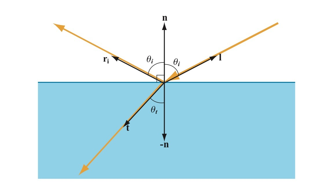
入射方向$\mathbf{l}$，反射方向$\mathbf{r} = 2(\mathbf{n} \cdot \mathbf{l})\mathbf{n} - \mathbf{l}$，法向量$\mathbf{n}$
漫射光和高光分别会根据入射方向、反射方向和观察方向的变化而变化，还可以通过$\alpha$参数来调节表面粗糙程度，从而控制高光区域大小和锐利程度，而且运算简单，适合当时的计算机处理能力。

Blinn-Phong Reflection Model

$I_{Blinn-Phong}=k_aI_a+k_d(n\cdot l)I_d+k_s(n\cdot h)^\alpha I_s$

半角向量$\mathbf{h}$为光线入射向量和观察向量的中间向量：$h=\frac{l+v}{||l+v||}$
Blinn-Phong相比Phong，在观察方向趋向平行于表面时，高光形状会拉长，更接近真实情况。

基于物理的分析模型

1967年Torrance-Sparrow在Theory for Off-Specular Reflection From Roughened Surfaces中使用辐射度学和微表面理论推导出粗糙表面的高光反射模型，1981年Cook-Torrance在A Reflectance Model for Computer Graphics中把这个模型引入到计算机图形学领域，现在无论是CG电影，还是3D游戏，基于物理着色都是使用的这个模型。Cook-Torrance：ROBERT L. COOK 和 KENNETH E. TORRANCE，提出这个BRDF的文章叫做《A Reflectance Model for Computer Graphics》，发表于1982年。

PBR 中的 Cook-Torrance BRDF 中，Cook-Torrance 是谁？ - 房燕良的回答 - 知乎 https://www.zhihu.com/question/351339310/answer/865238779

辐射度学（Radiometry）是度量电磁辐射能量传输的学科，也是基于物理着色模型的基础。
- 能量（Energy）$Q$，单位焦耳（$J$），每个光子都具有一定量的能量，和频率相关，频率越高，能量也越高，(波长越短)。
- 功率（Power），单位瓦特（Watts），或者焦耳／秒（J/s）。
  - 辐射度学中，辐射功率也被称为辐射通量（Radiant Flux）或者通量（Flux），指单位时间内通过表面或者空间区域的能量的总量，用符号$Φ$表示：$\Phi={\frac{dQ}{dt}}。$
- 辐照度（Irradiance），单位时间内到达单位面积的辐射能量，或到达单位面积的辐射通量。单位$W/m^2$ ，$E={\frac{d\Phi}{dA}}。$辐照度衡量的是到达表面的通量密度
- 辐出度（Radiant Existance），辐出度衡量的是离开表面的通量密度
  - 辐照度和辐出度都可以称为辐射通量密度（Radiant Flux Density）离光源越远，通量密度越低
- 辐射强度
  - 立体角（Solid Angle）立体角则是度量三维角度的量，用符号$\omega$表示，单位为立体弧度（也叫球面度，Steradian，简写为sr）等于立体角在单位球上对应的区域的面积（实际上也就是在任意半径的球上的面积除以半径的平方$\omega=\frac{s}{r^{2}}$），单位球的表面积是$4\pi$，所以整个球面的立体角也是$4\pi$。
  - 我们可以用一个向量和一个立体角来表示一束光线，向量表示这束光线的指向，立体角表示这束光线投射在单位球上的面积，也就是光束的粗细。
  - 辐射强度（Radiant Intensity），指通过单位立体角的辐射通量。用符号$I$表示，单位W/sr，定义为$I=\frac{d\Phi}{d\omega}$
  - 辐射强度不会随距离变化而变化，不像点光源的辐照度会随距离增大而衰减，这是因为立体角不会随距离变化而变化。
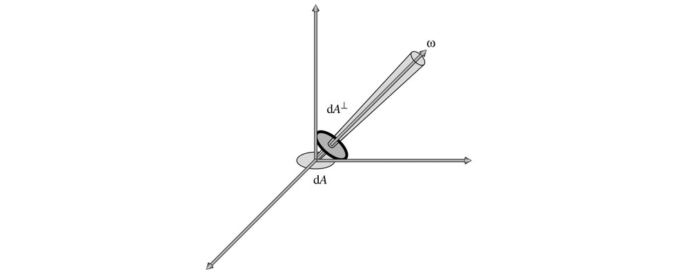
- 辐射率（Radiance），指每单位面积每单位立体角的辐射通量密度。用符号$L$表示，单位$W/m^{2}sr$，$L=\frac{d\Phi}{d\omega dA^{\perp}}$其中$dA^{\perp}$⊥是微分面积$dA$在垂直于光线方向的投影，如下图所示
  - 辐射率实际上可以看成是我们眼睛看到（或相机拍到）的物体上一点的颜色。在基于物理着色时，计算表面一点的颜色就是计算它的辐射率。
  - 辐射率不会随距离变化而衰减，这和我们日常感受一致，在没有雾霾的干扰时，我们看到的物体表面上一点的颜色并不会随距离变化而变化。为什么辐照度会随距离增大而衰减，但是我们看到的颜色却不会衰减呢？这是因为随着距离变大，我们看到的物体上的一块区域到达视网膜的通量密度会变小，同时这块区域在视网膜表面上的立体角也会变小，正好抵消了通量密度的变化。

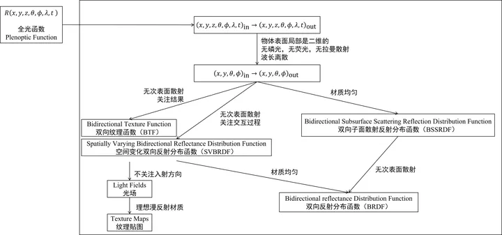
BRDF

我们看到一个表面，实际上是周围环境的光照射到表面上，然后表面将一部分光反射到我们眼睛里，双向反射分布函数BRDF（Bidirectional Reflectance Distribution Function）是描述表面入射光和反射光关系的。

对于一个方向的入射光，表面会将光反射到表面上半球的各个方向，不同方向反射的比例是不同的，我们用BRDF来表示指定方向的反射光和入射光的比例关系

$f(l,v)=\frac{dL_{o}(v)}{dE(l)}$

$l$是入射光方向，$v$是观察方向，也就是我们关心的反射光方向。
$dL_{o}(v)$是表面反射到$v$方向的反射光的微分辐射率。表面反射到$v$方向的反射光的辐射率为$L_{o}(v)$，来自于表面上半球所有方向的入射光线的贡献，而微分辐射率$dL_{o}(v)$特指来自方向$l$的入射光贡献的反射辐射率。$W/m^{2}sr$
$dE(l)$是表面上来自入射光方向$l$的微分辐照度。表面接收到的辐照度为$E(l)$，来自上半球所有方向的入射光线的贡献，而微分辐照度$dE(l)$特指来自于方向$l$的入射光。$W/m^2$
BRDF：f单位为$\frac{1}{sr}$

(32 封私信 / 44 条消息) brdf为什么要定义为一个单位是sr-1的量？ - 知乎 (zhihu.com)

表面对不同频率的光反射率可能不一样，因此BRDF和光的频率有关。在图形学中，将BRDF表示为RGB向量，三个分量各有自己的$f$函数

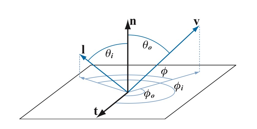
BRDF需要处理表面上半球的各个方向，如下图使用球坐标系定义方向更加方便。球坐标系使用两个角度来确定一个方向：

方向相对法线的角度$\theta$，称为极角（Polar Angle）或天顶角（Zenith Angle）
方向在平面上的投影相对于平面上一个坐标轴的角度$\phi$，称为方位角（Azimuthal Angle）

因此BRDF也可以写成：$f(\theta_i,\phi_i,\theta_o,\phi_o)$

怎么用BRDF来计算表面辐射率

来自方向$l$的入射辐射率：$L_i(l)=\frac{d\Phi}{d\omega_idA^-}=\frac{d\Phi}{d\omega_idAcos\theta_i}=\frac{dE(l)}{d\omega_icos\theta_i}$
则照射到表面来自于方向$l$的入射光贡献的微分辐照度：$dE(l)=L_i(l)d\omega_icos\theta_i$

表面反射到$v$方向的由来自于方向$l$的入射光贡献的微分辐射率：$dL_o(v)=f(l,v)\otimes dE(l)=f(l,v)\otimes L_i(l)d\omega_icos\theta_i$
要计算表面反射到$v$方向的来自上半球所有方向入射光线贡献的辐射率，可以将上式对半球所有方向的光线积分：$L_{o}(v)=\int_{\Omega}f(l,v)\otimes L_{i}(l)cos\theta_{i}d\omega_{i}$(表面反射辐射率即方向$v$观察到的颜色)

对于点光源、方向光等理想化的精准光源（Punctual Light），计算过程可以大大简化。我们考察单个精准光源照射表面，此时表面上的一点只会被来自一个方向的一条光线照射到（而面积光源照射表面时，表面上一点会被来自多个方向的多条光线照射到），则辐射率：$L_o(v)=f(l,v)\otimes E_Lcos\theta_i$，or多条光线：$L_{o}(v)=\sum_{k=1}^{n}f(l_{k},v)\otimes E_{L_{k}}cos\theta_{i_{k}}$

这里使用光源的辐照度，对于阳光等全局方向光，可以认为整个场景的辐照度是一个常数，对于点光源，辐照度随距离的平方衰减，用公式$E_{L}=\frac{\Phi}{4\pi r^{2}}$就可以求出到达表面的辐照度，Φ是光源的功率，比如100瓦的灯泡，r是表面离光源的距离

BRDF（Microfacet Theory）

我们用法线分布函数（Normal Distribution Function，简写为NDF）D(h)来描述组成表面一点的所有微表面的法线分布概率，现在可以这样理解：向NDF输入一个朝向ℎ，NDF会返回朝向是ℎ的微表面数占微表面总数的比例（虽然实际并不是这样，这点我们在讲推导过程的时候再讲），比如有1%的微表面朝向是ℎ，那么就有1%的微表面可能将光线反射到v方向。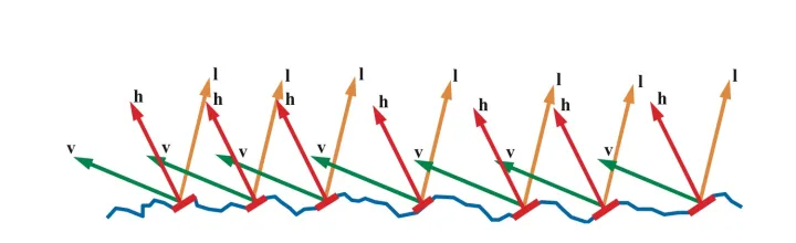

实际上并不是所有微表面都能收到接受到光线，如下面左边的图有一部分入射光线被遮挡住，这种现象称为Shadowing。也不是所有反射光线都能到达眼睛，下面中间的图，一部分反射光线被遮挡住了，这种现象称为Masking。光线在微表面之间还会互相反射，如下面右边的图，这可能也是一部分漫射光的来源，在建模高光时忽略掉这部分光线。

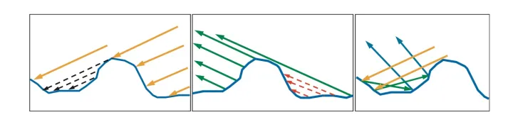
Shadowing和Masking用几何衰减因子（Geometrical Attenuation Factor）$G(l,v)$来建模，输入入射和出射光线方向，输出值表示光线未被遮蔽而能从$l$反射到$v$方向的比例
光学平面并不会将所有光线都反射掉，而是一部分被反射，一部分被折射，反射比例符合菲涅尔方程（Fresnel Equations）$F(l,h)$

则BRDF镜面反射部分：
$f(l,v)=\frac{F(l,h)G(l,v)D(h)}{4cos\theta_icos\theta_o}=\frac{F(l,h)G(l,v)D(h)}{4(n\cdot l)(n\cdot v)}$

n为宏观表面法线
h为微表面法线

为什么BRDF的漫反射项要除以π？ - 知乎 (zhihu.com)

光照模型有很多种1，Cook-Torrance 光照模型是最常用的。光照一般划分为漫反射和高光。漫反射模型提出的有 Lambert、 Oren-Nayar、Minnaert 三种，它们有着不同的计算公式。Cook-Torrance 采用 Lambert 漫反射后的计算如下：
$f=k_{d}f_{lambert}+k_{s}f_{cook-torrance},\quad f_{lambert}=\frac{c_{diffuse}}{\pi}$

反照率（albedo）是行星物理学中用来表示天体反射本领的物理量，定义为物体的辐射度（radiosity）与辐照度（irradiance）之比。射是出，照是入，出射量除以入射量，得到无量纲量。绝对黑体（black body）的反照率是0。煤炭呈黑色，反照率接近0，因为它吸收了投射到其表面上的几乎所有可见光。镜面将可见光几乎全部反射出去，其反照率接近1。albedo 翻译成反照率，与 reflectance（反射率）是有区别的。反射率用来表示某一种波长的反射能量与入射能量之比；而反照率用来表示全波段的反射能量与入射能量之比。BRDF 的 R 是 reflectance，方程仅关注一种波长。

NeRO中的BRDF

$f(\omega_{i},\omega_{0})=\underbrace{(1-m)\frac{a}{\pi}}_{\mathrm{diffuse}}+\underbrace{\frac{DFG}{4(\omega_{i}\cdot\mathbf{n})(\omega_{0}\cdot\mathbf{n})}}_{\mathrm{specular}},$

Specular

微面BRDF，参考上

Diffuse

Physically Based Rendering - 就决定是你了 | Ciel’s Blog (ciel1012.github.io)

specular用于描述光线击中物体表面后直接反射回去，使表面看起来像一面镜子。有些光会透入被照明物体的内部。这些光线要么被物体吸收（通常转换为热量），要么在物体内被散射。有一些散射光线有可能会返回表面，被眼球或相机捕捉到，这就是diffuse light。diffuse和subsurface scattering(次表面散射)描述的都是同一个现象。
根据材质，吸收和散射的光通常具有不同波长，因此仅有部分光被吸收，使得物体具有了颜色。散射通常是方向随机的，具有各向同性。使用这种近似的着色器只需要输入一个反照率(albedo)，用来描述从表面散射回来的各种颜色的光的分量。Diffuse color有时是一个同义词。

镜面反射和漫反射是互相排斥的。这是因为，如果一个光线想要漫反射，它必须先透射进材质里，也就是说，没有被镜面反射。这在着色语言中被称为“Energy Conservation（能量守恒）”，意思是一束光线在射出表面以后绝对不会比射入表面时更亮。

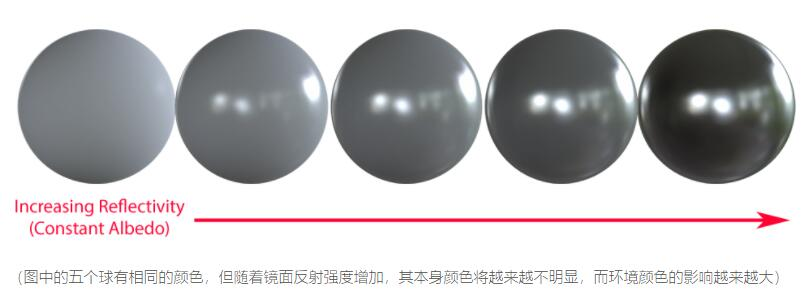
金属度相当于镜面反射，金属度越高，镜面反射越强

采样方式

将像素看成一个点，射出的光线是一条直线

(NerfAcc)可大致分为：

平均采样(粗采样)
空间跳跃采样(NGP中对空气跳过采样)
逆变换采样(根据粗采样得到的w分布进行精采样)

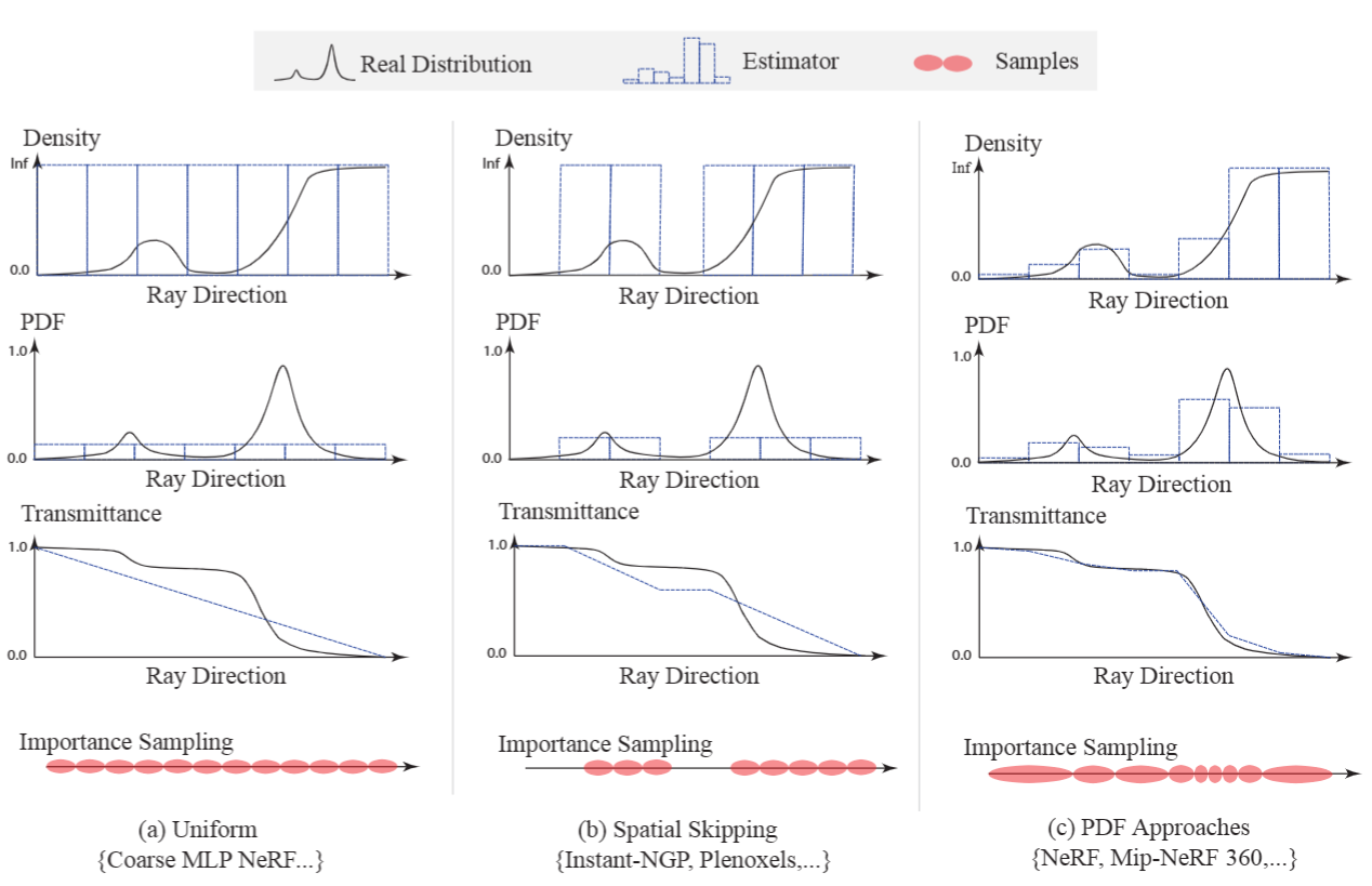
平均采样

i.e. 粗采样，在光线上平均采样n个点

占据采样

Occupancy Grids
通过在某分辨率占用网格中进行更新占用网格的权重，来确定哪些网格需要采样

逆变换采样

NeRF

简单的逆变换采样方法：根据粗采样得到的权重进行逆变换采样，获取精采样点
逆变换采样 - 知乎 (zhihu.com)

def sample_pdf(bins, weights, N_samples, det=False, pytest=False):
    # Get pdf
    weights = weights + 1e-5 # prevent nans # weights : chunk * 62

    # 归一化weights
    pdf = weights / torch.sum(weights, -1, keepdim=True) # pdf : chunk * 62
    cdf = torch.cumsum(pdf, -1) # cdf : chunk * 62
    cdf = torch.cat([torch.zeros_like(cdf[...,:1]), cdf], -1)  # (batch, len(bins))  = (chunk, 63)

    # Take uniform samples
    if det:
        u = torch.linspace(0., 1., steps=N_samples)
        u = u.expand(list(cdf.shape[:-1]) + [N_samples]) # u : chunk * N_samples
    else:
        u = torch.rand(list(cdf.shape[:-1]) + [N_samples])

    # Pytest, overwrite u with numpy's fixed random numbers
    if pytest:
        np.random.seed(0)
        new_shape = list(cdf.shape[:-1]) + [N_samples] # new_shape : chunk * N_samples
        if det:
            u = np.linspace(0., 1., N_samples)
            u = np.broadcast_to(u, new_shape) # u : chunk * N_samples
        else:
            u = np.random.rand(*new_shape)
        u = torch.Tensor(u)

    # Invert CDF
    u = u.contiguous() # 确保张量在内存中是连续存储的
    # inds : chunk * N_samples
    inds = torch.searchsorted(cdf, u, right=True) # 将u中的元素在cdf中进行二分查找，返回其索引
    below = torch.max(torch.zeros_like(inds-1), inds-1) # below : chunk * N_samples
    above = torch.min((cdf.shape[-1]-1) * torch.ones_like(inds), inds) # above : chunk * N_samples
    inds_g = torch.stack([below, above], -1)  # (batch, N_samples, 2)

    # cdf_g = tf.gather(cdf, inds_g, axis=-1, batch_dims=len(inds_g.shape)-2)
    # bins_g = tf.gather(bins, inds_g, axis=-1, batch_dims=len(inds_g.shape)-2)
    matched_shape = [inds_g.shape[0], inds_g.shape[1], cdf.shape[-1]]  # (batch, N_samples, 63)
    cdf_g = torch.gather(cdf.unsqueeze(1).expand(matched_shape), 2, inds_g) 
    # unsqueeze(1) : (batch, 1, 63)
    # expand : (batch, N_samples, 63)
    # cdf_g : (batch, N_samples, 2)    
    bins_g = torch.gather(bins.unsqueeze(1).expand(matched_shape), 2, inds_g)

    denom = (cdf_g[...,1]-cdf_g[...,0]) # denom : chunk * N_samples
    # 如果denom小于1e-5，就用1代替
    denom = torch.where(denom<1e-5, torch.ones_like(denom), denom)
    t = (u-cdf_g[...,0])/denom
    samples = bins_g[...,0] + t * (bins_g[...,1]-bins_g[...,0])

    return samples # samples : chunk * N_samples

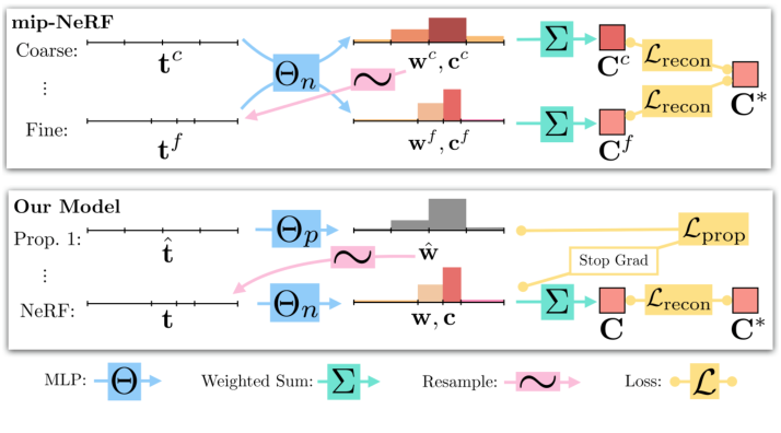
Mip-NeRF360

构建了一个提议网格获取权重来进行精采样（下）

锥形光线采样

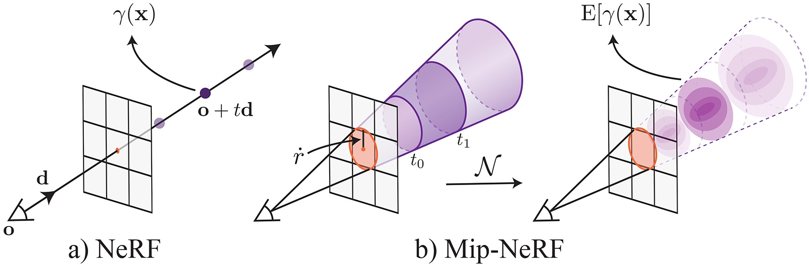
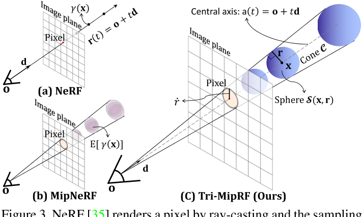
Mip-NeRF

将像素看成有面积的圆盘，射出的光线为一个圆锥体

使用多元高斯分布来近似截锥体

Tri-MipRF

使用一个各项同性的球来近似截锥体

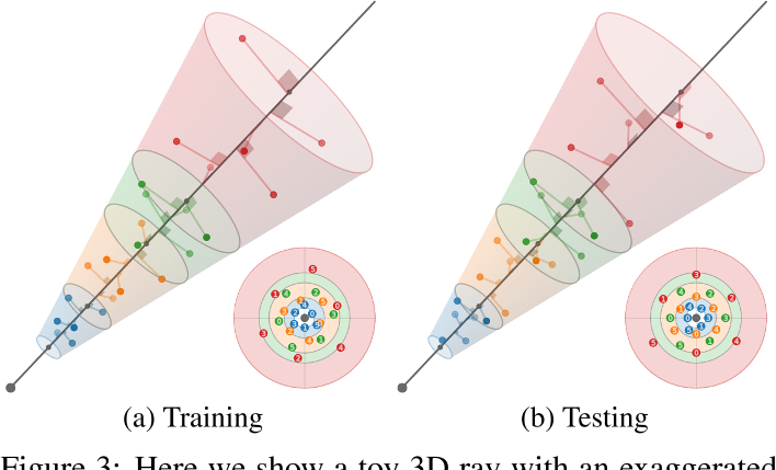
Zip-NeRF

Multisampling

多采样：在一个截锥体中沿着光线采样6个点，每个点之间旋转一个角度

对输入x进行编码的方式
Field Encoders - nerfstudio

编码方式

频率编码

NeRF from Scratch. Motivating the explanation from… | by Raja Parikshat | Medium 入门
Fourier Features Let Networks Learn High Frequency Functions in Low Dimensional Domains

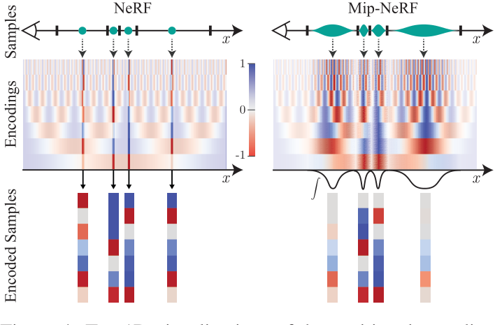
Frequency Encoding(Fourier Features), 作用：神经网络偏向于学习低频，提出的解决方案是使用位置编码，使用高频函数把输入映射到更高维的空间中，再传递到神经网络，可以更好地拟合具有高频变化的数据。
$\gamma(p)=\left(\sin \left(2^{0} \pi p\right), \cos \left(2^{0} \pi p\right), \cdots, \sin \left(2^{L-1} \pi p\right), \cos \left(2^{L-1} \pi p\right)\right)$

$p=x|y|z$
$L= constant$

NeRF

$\gamma(p)=\left(\sin \left(2^{0} \pi p\right), \cos \left(2^{0} \pi p\right), \cdots, \sin \left(2^{L-1} \pi p\right), \cos \left(2^{L-1} \pi p\right)\right)$

class Embedder:
    def __init__(self, **kwargs):
        self.kwargs = kwargs
        self.create_embedding_fn()

    def create_embedding_fn(self):
        embed_fns = []
        d = self.kwargs['input_dims']
        out_dim = 0
        if self.kwargs['include_input']:
            embed_fns.append(lambda x: x)
            out_dim += d

        max_freq = self.kwargs['max_freq_log2']
        N_freqs = self.kwargs['num_freqs']

        if self.kwargs['log_sampling']:
            freq_bands = 2. ** torch.linspace(0., max_freq, N_freqs)
        else:
            freq_bands = torch.linspace(2.**0., 2.**max_freq, N_freqs)

        for freq in freq_bands:
            for p_fn in self.kwargs['periodic_fns']:
                embed_fns.append(lambda x, p_fn=p_fn, freq=freq: p_fn(x * freq))
                out_dim += d

        self.embed_fns = embed_fns
        self.out_dim = out_dim

    def embed(self, inputs):
        return torch.cat([fn(inputs) for fn in self.embed_fns], -1)


def get_embedder(multires, input_dims=3):
    embed_kwargs = {
        'include_input': True,
        'input_dims': input_dims,
        'max_freq_log2': multires-1,
        'num_freqs': multires,
        'log_sampling': True,
        'periodic_fns': [torch.sin, torch.cos],
    }

    embedder_obj = Embedder(**embed_kwargs)
    def embed(x, eo=embedder_obj): return eo.embed(x)
    return embed, embedder_obj.out_dim

# multires <=> L
# use: get_embedder(args.multires, args.i_embed)

IPE

Mip-NeRF集成位置编码

对多元高斯近似截锥体的均值和协方差进行编码

$\begin{aligned} \gamma(\mathbf{\mu},\mathbf{\Sigma})& =\mathrm{E}_{\mathbf{x}\sim\mathcal{N}(\mathbf{\mu}_\gamma,\mathbf{\Sigma}_\gamma)}[\gamma(\mathbf{x})] \\ &=\begin{bmatrix}\sin(\mathbf{\mu}_\gamma)\circ\exp(-(1/2)\mathrm{diag}(\mathbf{\Sigma}_\gamma))\\\cos(\mathbf{\mu}_\gamma)\circ\exp(-(1/2)\mathrm{diag}(\mathbf{\Sigma}_\gamma))\end{bmatrix} \end{aligned}$

IPE可以将大区域的高频编码求和为0

多分辨率哈希编码

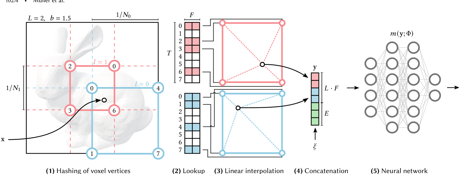
hashgrid.py:
class HashGrid(nn.Module):
    def __init__(self, n_input_dims, config):
        super().__init__()
        self.n_input_dims = n_input_dims
        with torch.cuda.device(get_rank()):
            self.encoding = tcnn.Encoding(self.n_input_dims, config_to_primitive(config))
        self.n_output_dims = self.encoding.n_output_dims
        self.n_level = config['n_levels']
        self.n_features_per_level = config['n_features_per_level']

    def forward(self, x):
        enc = self.encoding(x)
        return enc

models/neus.py：
class N(nn.Module):
    __init__:
    self.encoding = get_encoding(n_input_dims = 3, config)
    forward:
    h = self.encoding(x)

yaml:
    xyz_encoding: 
      otype: HashGrid
      n_levels: 16
      n_features_per_level: 2
      log2_hashmap_size: 19
      base_resolution: 16
      per_level_scale: 1.447269237440378
      include_xyz: true

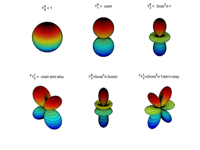
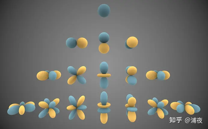
球面谐波编码

球面基函数——球谐函数

球谐函数介绍（Spherical Harmonics） - 知乎 (zhihu.com)

$\{Y_\ell^m\}.$ 与二维的三角函数基类似，球面谐波为三维上的一组基函数，用来描述其他更加复杂的函数

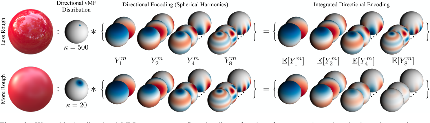
$\begin{aligned} y_l^m(\theta,\varphi)=\begin{cases}\sqrt{2}K_l^m\cos(m\varphi)P_l^m\big(\cos\theta\big),&m>0\\[2ex]\sqrt{2}K_l^m\sin(-m\varphi)P_l^{-m}\big(\cos\theta\big),&m<0\\[2ex]K_l^0P_l^0\big(\cos\theta\big),&m=0\end{cases} \\ P_n(x)=\frac1{2^n\cdot n!}\frac{d^n}{dx^n}[(x^2-1)^n] \\ P_l^m(x)=(-1)^m(1-x^2)^{m/2}\frac{d^m}{dx^m}(P_l(x)) \\ K_{l}^{m}=\sqrt{\frac{\left(2l+1\right)}{4\pi}\frac{\left(l-\left|m\right|\right)!}{\left(l+\left|m\right|\right)!}} \end{aligned}$

IDE

在Ref-NeRF中，借鉴Mip-NeR中的IPE，提出了IDE，基于球面谐波，将高频部分的编码输出置为0

$\mathrm{IDE}(\hat{\boldsymbol{\omega}}_r,\kappa)=\left\{\mathbb{E}_{\hat{\boldsymbol{\omega}}\sim\mathrm{vMF}(\hat{\boldsymbol{\omega}}_r,\kappa)}[Y_\ell^m(\hat{\boldsymbol{\omega}})]\colon(\ell,m)\in\mathcal{M}_L\right\},$
$\mathcal{M}_{L}=\{(\ell,m):\ell=1,…,2^{L},m=0,…,\ell\}.$

$\mathbb{E}_{\hat{\boldsymbol{\omega}}\sim\mathrm{vMF}(\hat{\boldsymbol{\omega}}_r,\kappa)}[Y_\ell^m(\hat{\boldsymbol{\omega}})]=A_\ell(\kappa)Y_\ell^m(\hat{\boldsymbol{\omega}}_r),$
$A_{\ell}(\kappa)\approx\exp\left(-\frac{\ell(\ell+1)}{2\kappa}\right).$

QiYun

Basics about 3D Reconstruction

Framework

体渲染函数

坐标变换

矩阵的QR分解

相机内参矩阵c2p

相机外参矩阵w2c

Neus(pose)

NeRO

镜面反射

Blinn-Phong Reflection Model

基于物理的分析模型

BRDF

BRDF（Microfacet Theory）

NeRO中的BRDF

Specular

Diffuse

采样方式

平均采样

占据采样

逆变换采样

NeRF

Mip-NeRF360

锥形光线采样

Mip-NeRF

Tri-MipRF

Zip-NeRF

编码方式

频率编码

NeRF

IPE

多分辨率哈希编码

球面谐波编码

IDE