| Title | Neuralangelo: High-Fidelity Neural Surface Reconstruction |
|---|---|
| Author | Zhaoshuo LiThomas MüllerAlex EvansRussell H. TaylorMathias UnberathMing-Yu LiuChen-Hsuan Lin |
| Conf/Jour | IEEE Conference on Computer Vision and Pattern Recognition (CVPR) |
| Year | 2023 |
| Project | Neuralangelo: High-Fidelity Neural Surface Reconstruction (nvidia.com) |
| Paper | Neuralangelo: High-Fidelity Neural Surface Reconstruction (readpaper.com) |
创新:新的计算梯度的方法——数值梯度、粗到精地逐步优化——数值梯度的补偿$\epsilon$,粗网格先激活,当$\epsilon$减小到精网格的空间大小时,逐步激活精网格
SR Issue: Current methods struggle to recover detailed structures of real-world scenes
To address : present Neuralangelo (combines the representation power of multi-resolution 3D hash grids with neural surface rendering)
- numerical gradients for computing higher-order derivatives as a smoothing operation
- coarse-to-fine optimization on the hash grids controlling different levels of details
even wo auxiliary inputs such as depth , Neuralangelo can effectively recover dense 3D surface structures from multi-view images with fidelity 保真 significantly surpassing previous methods, enabling detailed large-scale scene reconstruction from RGB video captures.
our future work to explore a more efficient sampling strategy to accelerate the training process.
实验
paper
数据集
- DTU dataset
- Tanks and Temples datase
实现细节
Our hash encoding resolution spans 25 to 211 with 16 levels. Each hash entry has a channel size of 8. The maximum number of hash entries of each resolution is 222.
We activate 4 and 8 hash resolutions at the beginning of optimization for DTU dataset and Tanks and Temples respectively, due to differences in scene scales. We enable a new hash resolution every 5000 iterations when the step size ε equals its grid cell size. For all experiments, we do not utilize auxiliary data such as segmentation(mask) or depth during the optimization process.
Evaluation criteria.
- Chamfer distance and F1 score for surface evaluation
- Large Scale Multi-view Stereopsis Evaluation-论文阅读讨论-ReadPaper
- Tanks and temples: benchmarking large-scale scene reconstruction-论文阅读讨论-ReadPaper
- Chamfer 距离越小,表示预测分割与真实分割越接近
- F1 得分的取值范围在 0 和 1 之间,越接近 1 表示模型的性能越好
- We use peak signal-tonoise ratio (PSNR) to report image synthesis qualities.
环境配置
数据集生成
colmap 数据生成
1 | DATA_PATH=datasets/${SEQUENCE}_ds${DOWNSAMPLE_RATE} |
or
1 | colmap gui Automatic reconstruction |
最后数据集:
1 | DATA_PATH |
1 | {DATA_PATH}/transforms.json |
SCENE_TYPE: can be one of{outdoor,indoor,object}.SEQUENCE: your custom name for the video sequence.
run
1 | EXPERIMENT=toy_example |
Isosurface extraction
1 | CHECKPOINT=logs/${GROUP}/${NAME}/xxx.pt |
- Add
--texturedto extract meshes with textures. - Add
--keep_lccto remove noises. May also remove thin structures. - Lower
BLOCK_RESto reduce GPU memory usage. - Lower
RESOLUTIONto reduce mesh size.
EXP
exp1
1 | # config gen |

Conclusion
We introduce Neuralangelo, an approach for photogrammetric neural surface reconstruction. The findings of Neuralangelo are simple yet effective: using numerical gradients for higher-order derivatives and a coarse-to-fine optimization strategy. Neuralangelo unlocks the representation power of multi-resolution hash encoding for neural surface reconstruction modeled as SDF. We show that Neuralangelo effectively recovers dense scene structures of both object-centric captures and large-scale indoor/outdoor scenes with extremely high fidelity, enabling detailed large-scale scene reconstruction from RGB videos. Our method currently samples pixels from images randomly without tracking their statistics and errors. Therefore, we use long training iterations to reduce the stochastics 随机指标 and ensure sufficient sampling of details. It is our future work to explore a more efficient sampling strategy to accelerate the training process.
AIR
The recovered surfaces provide structural information useful for many downstream applications,eg:
- 3D asset generation for augmented/virtual/mixed reality——AR/VR/MR 的 3D 资产生成
- environment mapping for autonomous navigation of robotics—— 机器人自主导航的环境映射
Photogrammetric surface reconstruction using a monocular RGB camera is of particular interest, as it equips users with the capability of casually 随意地 creating digital twins of the real world using ubiquitous mobile devices.
Multi-view stereo algorithms had been the method of choice for sparse 3D reconstruction,but an inherent drawback of these algorithms is their inability to handle ambiguous observations
- regions with large areas of homogeneous colors
- repetitive texture patterns
- strong color variations
This would result in inaccurate reconstructions with noisy or missing surfaces.
Recenty, neural surface reconstruction methods have shown great potential in addressing these limitations. Despite the superiority of neural surface reconstruction methods over classical approaches, the recovered fidelity of current methods does not scale well with the capacity of MLPs. 恢复的保真度不能很好地与 MLP 的容量进行 scale
Instant NGP introduces a hybrid 3D grid structure with a multi-resolution hash encoding and a lightweight MLP that is more expressive with a memory footprint loglinear to the resolution. NGP 的内存占用与分辨率 log 线性相关
本文 Neuralangelo = InstantNGP + Neus
Neuralangelo adopts Instant NGP as a neural SDF representation of the underlying 3D scene, optimized from multi-view image observations via neural surface rendering
Step:
- First, using numerical gradients to compute higher-order derivatives, such as surface normals for the eikonal regularization, is critical to stabilizing the optimization.
- Second, a progressive optimization schedule plays an important role in recovering the structures at different levels of details
We combine these two key ingredients and, via extensive experiments on standard benchmarks and real-world scenes, demonstrate significant improvements over image-based neural surface reconstruction methods inboth reconstruction accuracy 重建精度 and view synthesis quality 视图合成质量.
In summary:
- We present the Neuralangelo framework to naturally incorporate the representation power of multi-resolution hash encoding into neural SDF representations.
- We present two simple techniques to improve the quality of hash-encoded surface reconstruction: higher-order derivatives with numerical gradients and coarse-to-fine optimization with a progressive level of details.
RelatedWork:
- Multi-view surface reconstruction
- volumetric occupancy grid to represent the scene: Each voxel is visited and marked occupied if strict color constancy between the corresponding projected image pixels is satisfied. The photometric consistency assumption 光度一致性假设 typically fails due to autoexposure 自动曝光 or non-Lambertian materials 非朗伯材料, which are ubiquitous in the real world. Relaxing such color constancy constraints across views is important for realistic 3D reconstruction
- Follow-up methods typically start with 3D point clouds from multi-view stereo techniques and then perform dense surface reconstruction. Reliance on the quality of the generated point clouds often leads to missing or noisy surfaces. Recent learning-based approaches augment the point cloud generation process with learned image features and cost volume construction(MVSnet, DeepMVS). _However, these approaches are inherently limited by 花费体积的分辨率 the resolution of the cost volume and fail to recover geometric details._
- NeRF
- NeRF achieves remarkable photorealistic view synthesis with view-dependent effects. NeRF encodes 3D scenes with an MLP mapping 3D spatial locations to color and volume density. These predictions are composited into pixel colors using neural volume rendering. A problem of NeRF and its variants , however, is the question of how an isosurface of the volume density could be defined to represent the underlying 3D geometry. NeRF 的问题就是等值面不好找。Current practice often relies on heuristic thresholding 启发式阈值 on the density values; due to insufficient constraints on the level sets, however, such surfaces are often noisy and may not model the scene structures accurately. _Therefore, more direct modeling of surfaces is preferred for photogrammetric surface reconstruction problems._
- Neural surface reconstruction
- For scene representations with better-defined 3D surfaces, implicit functions such as occupancy grids(UNISURF) or SDFs are preferred over simple volume density fields.To integrate with neural volume rendering [25], different techniques [41, 47] have been proposed to reparametrize the underlying representations back to volume density 将底层表征重新参数化回体密度.These designs of neural implicit functions enable more accurate surface prediction with view synthesis capabilities of unsacrificed quality.
- Follow-up works extend the above approaches to realtime at the cost of surface fidelity 有牺牲保真度来实现实时建模的研究(Vox-Surf, Neus2), while others use auxiliary information to enhance the reconstruction results 其他的使用辅助信息增强重建结果(with patch warping, Geo-Nues, MonoSDF).
- Notably, NeuralWarp uses patch warping given co-visibility information from structure-frommotion (SfM) to guide surface optimization, but the patchwise planar assumption fails to capture highly-varying surfaces 补丁平面假设无法捕捉高度变化的表面.
- Other methods utilize sparse point clouds from SfM to supervise the SDF, but their performances are upper-bounded by the quality of the point clouds, as with classical approaches
- The use of depth and segmentation as auxiliary data has also been explored with unconstrained image collections or using scene representations with hash encodings.
- In contrast, our work Neuralangelo builds upon hash encodings to recover surfaces but without the need for auxiliary inputs used in prior work,本文的方法不需要输入一些辅助数据
- Concurrent work also proposes coarse-to-fine optimization for improved surface details, where a displacement network corrects the shape predicted by a coarse network,并行的方法,使用位移网络来纠错粗网络预测的形状
- In contrast, we use hierarchical hash grids and control the level of details based on our analysis of higher-order derivatives. 通过基于对高阶导数的分析来控制细节的级别
Approach
Neuralangelo reconstructs dense structures of the scene from multi-view images. Neuralangelo samples 3D locations along camera view directions and uses a multi-resolution hash encoding to encode the positions. The encoded features are input to an SDF MLP and a color MLP to composite images using SDF-based volume rendering.
3D 位置—>哈希编码后的位置信息—>SDF/Color
Preliminaries
- Neural volume rendering.
- Volume rendering of SDF
- Multi-resolution hash encoding
- 也有一种方式是 sparse voxel 结构,但是由于内存随着分辨率的增加呈现立方增长,太费内存占用,Hash encoding instead assumes no spatial hierarchy 空间层次结构 and resolves collision automatically based on gradient averaging 梯度平均
Numerical Gradient Computation

w.r.t. : with respect to 相对于,就…而言
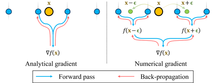
We show in this section that the analytical gradient w.r.t. position of hash encoding suffers from localities. 相对于哈希编码位置,解析梯度受到局部性的影响 . Therefore, optimization updates only propagate to local hash grids, lacking non-local smoothness. We propose a simple fix to such a locality problem by using numerical gradients. ???差分类似
A special property of SDF is its differentiability with a gradient of the unit norm. The gradient of SDF satisfies the eikonal equation $∥∇f (x)∥_{2} = 1$ (almost everywhere). To enforce the optimized neural representation to be a valid SDF, the eikonal loss is typically imposed on the SDF predictions:
由于 SDF 梯度在每处都满足二范数等于 1,因此构建 Eikonal loss 来优化 SDF 的预测:
$\mathcal{L}_{\mathrm{eik}}=\frac{1}{N}\sum_{i=1}^{N}(|\nabla f(\mathbf{x}_i)|_2-1)^2,$N 是总采样点数
To allow for end-to-end optimization, a double backward operation on the SDF prediction f (x) is required.
de-facto 先前的大部分方法
eikonal loss 反向传播到局部的哈希表项
The $de facto$ method for computing surface normals of SDFs ∇f (x) is to use analytical gradients. Analytical gradients of hash encoding w.r.t. position, however, are not continuous across space under trilinear interpolation. 哈希编码三线性插值下,哈希编码的解析梯度相对于位置在空间上是不连续的。
To find the sampling location in a voxel grid, each 3D point $x_{i}$ would first be scaled by the grid resolution $V_{l}$, written as $x_{i,l} = x_{i} · V_{l}.$ Let the coefficient for (tri-)linear interpolation be $β = x_{i,l} − ⌊x_{i,l}⌋$. The resulting feature vectors are
$\gamma_l(\mathbf{x}_{i,l})=\gamma_l(\lfloor\mathbf{x}_{i,l}\rfloor)\cdot(1-\beta)+\gamma_l(\lceil\mathbf{x}_{i,l}\rceil)\cdot\beta,$ where the rounded position$⌊x_{i,l⌋}, ⌈x_{i,l}⌉$correspond to the local grid cell corners. We note that rounding operations ⌊·⌋and ⌈·⌉ are non-differentiable, rounding 运算是不可微的,可以得到哈希编码相对于位置的微分:
The derivative of hash encoding is local, i.e., when $x_{i}$ moves across grid cell borders, the corresponding hash entries will be different. Therefore, the eikonal loss defined in Eq. 5 only back-propagates to the locally sampled hash entries, i.e. $γl(⌊x_{i,l}⌋) and γl(⌈x_{i,l}⌉)$. When continuous surfaces (e.g. a flat wall) span multiple grid cells, these grid cells should produce coherent surface normals without sudden transitions. 当表面连续或者很大,跨过多个网格单元时,这些网格单元应该产生连贯的表面法线,而不会突然转变,为了确保表面表示的一致性,应对这些网格单元联合优化,但是分析梯度仅仅只局限于局部网格单元。To ensure consistency in surface representation, joint optimization of these grid cells is desirable. However, the analytical gradient is limited to local grid cells, unless all corresponding grid cells happen to be sampled and optimized simultaneously. Such sampling is not always guaranteed
our method
To overcome the locality of the analytical gradient of hash encoding, we propose to compute the surface normals using numerical gradients.
If the step size of the numerical gradient is smaller than the grid size of hash encoding, the numerical gradient would be equivalent to the analytical gradient; otherwise, hash entries of multiple grid cells would participate in the surface normal computation.
- math 表达上面的描述 - step size < grid size :numerical gradient = analytical gradient - step size > grid size :多个网格的哈希表项都参与表面法向的计算
Backpropagating through the surface normals thus allows hash entries of multiple grids to receive optimization updates simultaneously. Intuitively, numerical gradients with carefully chosen step sizes can be interpreted as a smoothing operation on the analytical gradient expression. numerical gradients 通过选择 step size 可以解释为 analytical gradient 表示的平滑操作
An alternative of normal supervision is a teacher-student curriculum(Ref-NeRF, NeRFactor), where the predicted noisy normals are driven towards MLP outputs to exploit the smoothness of MLPs 利用 MLP 的平滑性,将预测的嘈杂法线作为 MLP 的输出,然而 loss 的解析梯度也只能反向传播到局部的单元网格来进行哈希编码. However, analytical gradients from such teacher-student losses still only back-propagate to local grid cells for hash encoding. In contrast, numerical gradients solve the locality issue without the need of additional networks.
To compute the surface normals using the numerical gradient, additional SDF samples are needed. Given a sampled point $x_{i} = (x_{i}, y_{i}, z_{i})$, we additionally sample two points along each axis of the canonical coordinate around xi within a vicinity 范围内 of a step size of ε. For example, the x-component of the surface normal can be found as:$\nabla_xf(\mathbf{x}_i)=\frac{f\left(\gamma(\mathbf{x}_i+\epsilon_x)\right)-f\left(\gamma(\mathbf{x}_i-\epsilon_x)\right)}{2\epsilon},$ $\epsilon_{x} = [\epsilon, 0, 0]$

Progressive Levels of Details
Coarse-to-fine optimization can better shape the loss landscape to avoid falling into false local minima. Such a strategy has found many applications in computer vision, such as image-based registration .
Neuralangelo also adopts a coarse-to-fine optimization scheme to reconstruct the surfaces with progressive levels of details. Using numerical gradients for the higher-order derivatives naturally enables Neuralangelo to perform coarse-to-fine optimization from two perspectives.
- Step size ε. As previously discussed, numerical gradients can be interpreted as a smoothing operation where the step size ε controls the resolution and the amount of recovered details. Imposing $\mathcal{L}_{eik}$ with a larger ε for numerical surface normal computation ensures the surface normal is consistent at a larger scale, thus producing consistent and continuous surfaces. On the other hand, imposing $\mathcal{L}_{eik}$ with a smaller ε affects a smaller region and avoids smoothing details. In practice, we initialize the step size ε to the coarsest hash grid size and exponentially decrease it matching different hash grid sizes throughout the optimization process. 初始化$\epsilon$ 为最粗的哈希网格大小,并在整个优化过程中匹配不同的网格大小,以指数方式减小它
- Hash grid resolution V . If all hash grids are activated from the start of the optimization, to capture geometric details, fine hash grids must first “unlearn” from the coarse optimization with large step size ε and “relearn” with a smaller ε. If such a process is unsuccessful due to converged optimization, geometric details would be lost. Therefore, we only enable an initial set of coarse hash grids and progressively activate finer hash grids throughout optimization when ε decreases to their spatial size. 粗网格先激活,当$\epsilon$减小到精网格的空间大小时,逐步激活精网格,可以更好的捕捉到细节。The relearning process can thus be avoided to better capture the details. In practice, we also apply weight decay over all parameters to avoid single-resolution features dominating the final results.
Optimization
To further encourage the smoothness of the reconstructed surfaces, we impose a prior by regularizing the mean curvature of SDF 通过正则化平均曲率施加先验
The mean curvature is computed from discrete Laplacian similar to the surface normal computation, otherwise, the second-order analytical gradients of hash encoding are zero everywhere when using trilinear interpolation. The curvature loss Lcurv is defined as:$\mathcal{L}_{\mathtt{curv}}=\frac{1}{N}\sum_{i=1}^{N}\left|\nabla^{2}f(\mathbf{x}_{i})\right|.$
We note that the samples used for the surface normal computation in Eq. 8:$\nabla_xf(\mathbf{x}_i)=\frac{f\left(\gamma(\mathbf{x}_i+\epsilon_x)\right)-f\left(\gamma(\mathbf{x}_i-\epsilon_x)\right)}{2\epsilon},$ are sufficient for curvature computation.
The total loss is defined as the weighted sum of losses:
$\mathcal{L}=\mathcal{L}_{\mathrm{RGB}}+w_{\mathrm{eik}}\mathcal{L}_{\mathrm{eik}}+w_{\mathrm{curv}}\mathcal{L}_{\mathrm{curv}}.$
All network parameters, including MLPs and hash encoding, are trained jointly end-to-end.所有网络参数,端到端的联合训练