- Accuracy 重建的模型精度不好,影响因素:
- 数据集质量:照片拍摄质量(设备)、相机位姿估计精度(COLMAP)
- 照片质量问题:混叠、模糊、滚动快门 (RS) 效应、HDR/LDR、运动模糊、低光照
- NeuS方法的问题:Loss函数约束、体渲染的过度简化、缺少监督(深度or法向量)
- 网格提取方法(Marching Cube)
- 数据集质量:照片拍摄质量(设备)、相机位姿估计精度(COLMAP)
- Efficiency 训练/渲染的速度太慢,影响因素:
- MLP计算次数多 —> MIMO MLP、NGP-RT、
- MLP层数多计算慢—> InstantNGP
IDEA
- 监督深度图信息
Accuracy
Camera Pose Estimation
3D Point Sampling
NerfAcc
NerfAcc:占据+逆变换采样 混合采样方式
先使用占据网格确定哪些区域需要采样,再通过粗采样得到的权重使用逆变换采样进行精采样得到采样点
Loss Function
S3IM
S3IM: Stochastic Structural SIMilarity and Its Unreasonable Effectiveness for Neural Fields
MSE loss 是 point-wise 的,没有考虑到一组pixel的结构特征,而SSIM通过一个KxK的核和stride扫过整个图像,最后求平均MSSIM,可以考虑图像的结构信息。
- $\mathrm{SSIM}(a,b)=l(\boldsymbol{a},\boldsymbol{b})c(\boldsymbol{a},\boldsymbol{b})s(\boldsymbol{a},\boldsymbol{b}).$ 一个核覆盖的图像,$C_{1},C_{2},C_{3}$ 是小的常数
- luminance亮度:$l(\boldsymbol{a},\boldsymbol{b})=\frac{2\mu_a\mu_b+C_1}{\mu_a^2+\mu_b^2+C_1},$
- contrast对比度:$c(\boldsymbol{a},\boldsymbol{b})=\frac{2\sigma_a\sigma_b+C_2}{\sigma_a^2+\sigma_b^2+C_2},$
- structure结构:$s(\boldsymbol{a},\boldsymbol{b})=\frac{\sigma_{ab}+C_3}{\sigma_a\sigma_b+C_3}.$
但是在NeRF训练过程中pixel在一个batch是随机的,丢失了局部patch的像素中位置相关的信息,本文提出的S3IM,是SSIM的随机变体。每个minibatch有B个像素,核大小KxK,步长s=K(因为在minibatch中的随机patch是独立的,而且不需要重叠的情况)
- 将B个像素/光线构成一个rendered patch $\mathcal{P}(\hat{\mathcal{C}})$,同时有一个gt image patch $\mathcal{P}(\mathcal{C})$
- 计算rendered和gt patch之间的$SSIM(\mathcal{P}(\hat{\mathcal{C}}),\mathcal{P}(\mathcal{C}))$ with kernel size KxK and stride size s =K
- 由于patch是随机的,重复M次上述两步,并计算M次SSIM的平均值
$\mathrm{S3IM}(\hat{\mathcal{R}},\mathcal{R})=\frac{1}{M}\sum_{m=1}^{M}\mathrm{SSIM}(\mathcal{P}^{(m)}(\hat{\mathcal{C}}),\mathcal{P}^{(m)}(\mathcal{C}))$
$L_{\mathrm{S3IM}}(\Theta,\mathcal{R})=1-\mathrm{S3IM}(\hat{\mathcal{R}},\mathcal{R}) = =1-\frac1M\sum_{m=1}^M\mathrm{SSIM}(\mathcal{P}^{(m)}(\hat{\mathcal{C}}),\mathcal{P}^{(m)}(\mathcal{C}))$
Volume Rendering
NeuS
NeuS: Learning Neural Implicit Surfaces by Volume Rendering for Multi-view Reconstruction
SDF内部-1,外部1,表面0
NeuS没有与NeRF一样直接使用MLP输出的不透明度$\sigma$作为$\rho$,而是使用预测的sdf进行相应计算得到$\rho$,以及权重
- $C(\mathbf{o},\mathbf{v})=\int_{0}^{+\infty}w(t)c(\mathbf{p}(t),\mathbf{v})\mathrm{d}t$ $\omega(t)=T(t)\rho(t),\text{where}T(t)=\exp\left(-\int_0^t\rho(u)\mathrm{d}u\right)$
- $\rho(t)=\max\left(\frac{-\frac{\mathrm{d}\Phi_s}{\mathrm{d}t}(f(\mathbf{p}(t)))}{\Phi_s(f(\mathbf{p}(t)))},0\right)$ , MLP预测的sdf即$f(\mathbf{p}(t))$
- $\phi_s(x) =\frac{se^{-sx}}{(1+e^{-sx})^{2}}$, $\Phi_s(x)=(1+e^{-sx})^{-1},\text{i.e.,}\phi_s(x)=\Phi_s’(x)$
离散化:
- $\hat{C}=\sum_{i=1}^nT_i\alpha_ic_i,$ $\alpha_i=1-\exp\left(-\int_{t_i}^{t_{i+1}}\rho(t)\mathrm{d}t\right),$ $T_i=\prod_{j=1}^{i-1}(1-\alpha_j)$
- $\alpha_i=\max\left(\frac{\Phi_s(f(\mathbf{p}(t_i)))-\Phi_s(f(\mathbf{p}(t_{i+1})))}{\Phi_s(f(\mathbf{p}(t_i)))},0\right).$
- $\alpha_{i}=max()$
除了$\mathcal{L}1$和$\mathcal{L}_{mask}$损失之外还使用了$\mathcal{L}_{r e g}=\frac{1}{n m}\sum_{k,i}(|\nabla f(\hat{\mathbf{p}}_{k,i})|_{2}-1)^{2}.$ (Eikonal term)
- where m is batch size(ray scalar), n is the point sampling size
NeuRodin
NeuRodin: A Two-stage Framework for High-Fidelity Neural Surface Reconstruction
室内外大场景,之前方法存在的问题:
- 过度几何正则化a);
- 没有对几何拓扑约束b);
- 本文Two-stage的想法:首先对SDF不进行约束(不用$\mathcal{L}_{eik}$,类似density进行训练),然后使用几何正则化来refine光滑表面
先前 SDF-based volume rendering 方法的不足:
- SDF到密度转换的不合适假设:$\sigma(\mathbf{r}(t))=\Psi_s(f(\mathbf{r}(t)))=\begin{cases}\frac{1}{2s}\exp\left(\frac{-f(\mathbf{r}(t))}{s}\right)&\text{if }f(\mathbf{r}(t))\geq0,\\\frac{1}{s}\left(1-\frac{1}{2}\exp\left(\frac{f(\mathbf{r}(t))}{s}\right)\right)&\text{if }f(\mathbf{r}(t))<0.\end{cases}$
- SDF值相同的区域密度值也是相同的,限制了密度场(derived from SDF)的表达能力。
- 原先的密度场方法(NeRF)的密度值范围可以是$[0,+\infty]$,而SDF计算得到的密度范围在$\left(0,\frac{1}{s} \right]$ Function Desmos
- 密度偏差(SDF to Density过程中),虽有很多改进但是偏差仍存在,且几何正则化会产生一些不好影响 (exacerbates this bias, complicating model convergence and resulting in the creation of inaccurate surfaces),一些改进的方法:
- TUVR: Towards Unbiased Volume Rendering of Neural Implicit Surfaces with Geometry Priors
- Debsdf: Delving into the details and bias of neural indoor scene reconstruction
- Recovering fine details for neural implicit surface reconstruction.
- 几何过度正则化,such as Eikonal loss or smoothness constraints,导致缺陷:
- 在所有区域过度光滑, both flat and intricate, leading to a loss of fine details)。
- 当优化Normal产生的颜色和通过几何正则化显式地约束SDF时,优化过程会阻碍拓扑结构的产生。
本文解决方法:
- Uniform SDF, Diverse Densities
- 空间中每一点都有独自的缩放因子:使用非线性映射来根据三维空间中一点坐标获取独一无二的缩放因子s (local scale $s(t)$) (类似Adaptive shells for efficient neural radiance field rendering.的工作,需要结合SDF和density的特性)
- $(f(\mathbf{r}(t)),s(\mathbf{r}(t)),\mathbf{z}(\mathbf{r}(t)))=\phi_\text{geo}(\mathbf{r}(t)),\quad\sigma(\mathbf{r}(t))=\Psi_{s(\mathbf{r}(t))}\left(f(\mathbf{r}(t))\right).$ 解释:(SDF, s, 几何特征)=非线性映射(点坐标) and 密度=函数(SDF, s)
- Explicit Bias Correction
- 存在的偏差
- A: maximum probability distance$\hat{D}_{\text{prob}}(\mathbf{r})=\arg\max_{t\in(0,+\infty)}w(t)=\arg\max_{t\in(0,+\infty)}T(t)\sigma(\mathbf{r}(t)).$
- B: rendered distance $\hat{D}_{\text{rendered}}(\mathbf{r})=\int_0^{+\infty}T(t)\sigma(\mathbf{r}(t))t \mathrm{d}t.$ 相当于对权重求了均值
- C: SDF zero level set
- 本文解决方法:
- 通过约束每条光线上A($t^*$ with bias correction factor $\epsilon_{\mathrm{bias}}$)与C的差异,且仅约束sdf为正(即模型外部)的部分
- 为什么不约束模型内部呢?:鼓励SDF在A位置之后取负值,经验测试出来的(附录C),且提供了数学解释: 当A在C之前时,随着$\theta$的变化AC之间差异变化的更大;当A在C之后时,随着$\theta$的变化AC之间差异变化较小
- $\epsilon_{\mathrm{bias}}$ 是由于选取maximum的方法导致的:直接使用采样点的最大权重来近似$t^*$
- 存在的偏差
- Two-Stage Optimization to Tackle Geometry Over-Regularization
- Stage 1——Geometry Over-Regularization (estimated gradients + local scale s(VolSDF SDF2Density) + $\mathcal{L}_{\mathrm{bias}}$)
- 直观解法:消除几何约束或者降低权重,且避免condition颜色(predicted normal)。 但是会产生非自然的SDF zero-level set
- 简单高效的解法是:不直接使用梯度${\nabla f(\mathbf{r}(t))}$进行几何正则,而是使用估计梯度$\hat{\nabla}f(\mathbf{r}(t))$通过特殊设计来引入不确定性,
- x分量的估计梯度为:$\hat{\nabla}_xf(\mathbf{r}(t))=\frac{f\left(\mathbf{r}(t)+\boldsymbol{\epsilon}_x\right)-f\left(\mathbf{r}(t)-\boldsymbol{\epsilon}_x\right)}{2\epsilon},\quad\text{where }\epsilon_x=(\epsilon,0,0)\text{ and }\epsilon\sim U(0,\epsilon_{\max}).$
- 通过有限差分法估计梯度的step size $\epsilon$是一个随机采样的数,这样在更大的场景的estimated normal中有很小的variance,在fine details的normal中有更大的variance。这样的不确定性确保了更大特征的稳定性和复杂细节的灵活性
- 总结:
- $\mathcal{L}_{\mathrm{coarse}}=\mathcal{L}_{\mathrm{color}}+\lambda_{\mathrm{eik}}\mathcal{L}_{\mathrm{eik}}(\hat{\nabla}f)+\lambda_{\mathrm{bias}}\mathcal{L}_{\mathrm{bias}}.$
- VolSDF的SDF-to-density方法:
- $\sigma(\mathbf{r}(t))=\Psi_s(f(\mathbf{r}(t)))=\begin{cases}\frac{1}{2s}\exp\left(\frac{-f(\mathbf{r}(t))}{s}\right)&\text{if }f(\mathbf{r}(t))\geq0,\\\frac{1}{s}\left(1-\frac{1}{2}\exp\left(\frac{f(\mathbf{r}(t))}{s}\right)\right)&\text{if }f(\mathbf{r}(t))<0.\end{cases}$
- Stage 2——Refinement (estimated gradients + TUVR SDF2Density + $\mathcal{L}_{\mathrm{smooth}}$)
- 使用PermutoSDF的损失$\mathcal{L}_{\mathrm{smooth}}=\frac1{mn}\sum_{\mathbf{r},t}\left(\mathbf{n}\left(\mathbf{r}(t)\right)\cdot\mathbf{n}\left(\mathbf{r}(t)+\epsilon_s\boldsymbol{\eta}(\mathbf{r}(t))\right)-1\right)^2,$ 来增加局部光滑度,$\boldsymbol{\eta}(\mathbf{r}(t)) = \mathbf{n}(\mathbf{r}(t)) \times \boldsymbol{\tau}$ 其中$\tau$是随机单位向量
- 总结:
- 采用TUVR的 SDF-to-density方法,保证最小化bias且保存fine的物体细节
- $\sigma(t)=\begin{cases}\frac{1}{s(t)}\exp\left(\frac{-f(t)}{s(t)|f’(t)|}\right)&\text{if}f(t)\geq0,\\\frac{2}{s(t)}\left(1-\frac{1}{2}\exp\left(\frac{f(t)}{s(t)|f’(t)|}\right)\right)&\text{if}f(t)<0.\end{cases}$
- $\mathcal{L}_{\mathrm{fine}}=\mathcal{L}_{\mathrm{color}}+\lambda_{\mathrm{eik}}\mathcal{L}_{\mathrm{eik}}(\nabla f)+\lambda_{\mathrm{smooth}}\mathcal{L}_{\mathrm{smooth}}.$
- 采用TUVR的 SDF-to-density方法,保证最小化bias且保存fine的物体细节
- Stage 1——Geometry Over-Regularization (estimated gradients + local scale s(VolSDF SDF2Density) + $\mathcal{L}_{\mathrm{bias}}$)
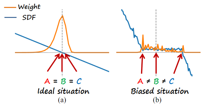
附录的理论分析:
- 根据权重最大的点$t^*=\arg\max_{t\in(0,+\infty)}T(t)\sigma(\mathbf{r}(t))$
- 在该点应该满足$\frac{\partial w(t)}{\partial t}\Bigg|_{t=t^*}=0$
- 可以推导出
因此构建的SDF-to-density函数必须满足:
- 条件1
- 条件2 (SDF=0的点,同时权重最大)
然而: - NeuS只有在沿着光线的SDF分布的一阶近似条件下才满足此条件
- TUVR扩展到了任意分布,但是仍有问题就是不一定$t^{0} \neq t^{*}$,(在优化过程中,沿着光线的权重分布是一个复杂的non-convex函数,只能担保$t^{0}$是在局部最大值上)
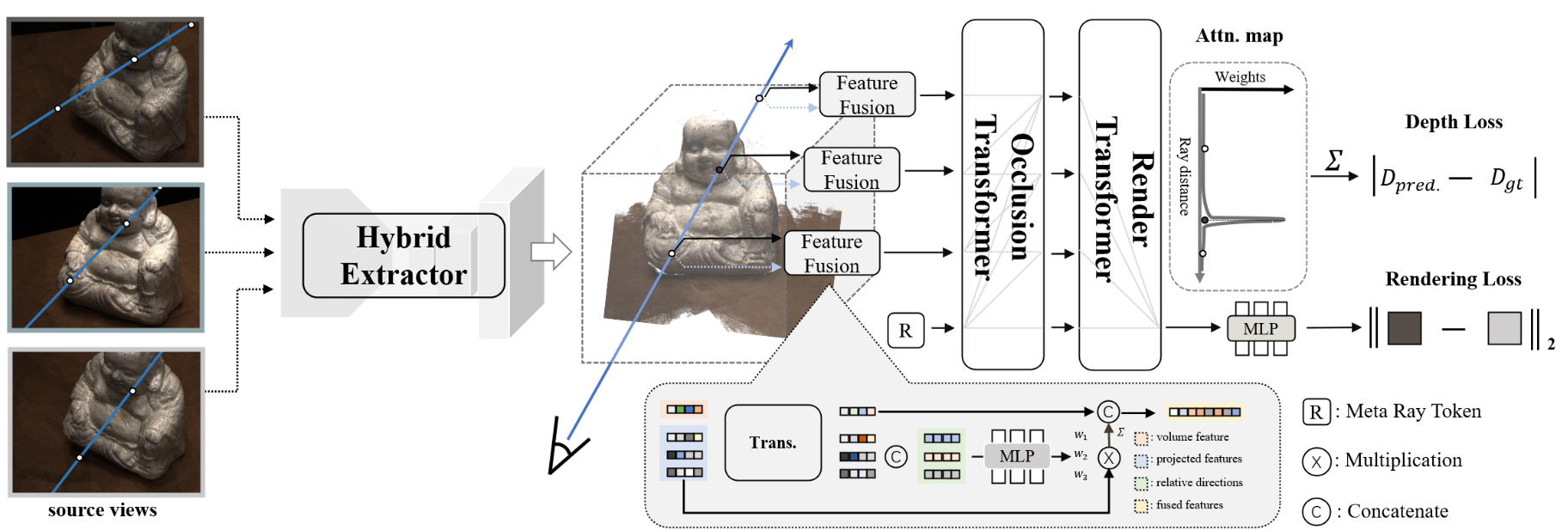
ReTR
ReTR: Modeling Rendering Via Transformer for Generalizable Neural Surface Reconstruction
使用Transformer 代替渲染过程,并且添加了深度监督
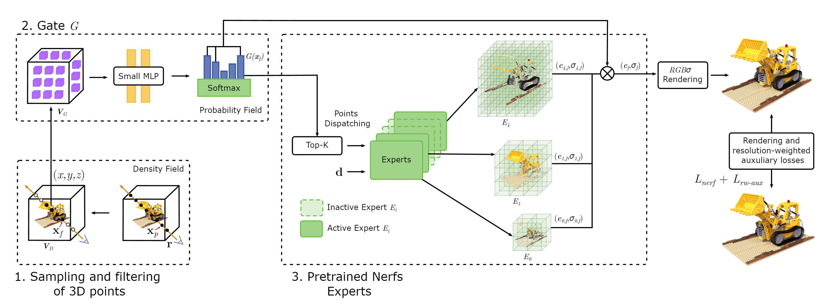
Mixture of Experts (MoE)
Boost Your NeRF
混合专家模型(MoE)详解 MoE 层由两个核心部分组成: 一个门控网络(用于决定哪些令牌 (token) 被发送到哪个专家)和若干数量的专家(每个专家本身是一个独立的神经网络)
- 门控网络来决定采样点被输入哪 Top-K个专家网络(并且在filtering step抛弃low-density的点,密度值根据lowest resolution model 进行计算)
- 每个专家网络以采样点位置和方向作为输入,输出颜色和密度
- 根据该点到每个专家网络的权重(概率Probability Field)和颜色密度值,计算该点最终的颜色和密度值。最后通过体渲染得到pixel color,并联合优化resolution-weighted auxiliary loss(用于选取专家网络)
主要思想是在训练了一批不同分辨率的NeRF models后,优先使用low-resolution models,减少high-resolution models 的使用
Efficiency
- 完全抛弃MLP,存储显示的颜色/密度
- 加速渲染:对几何代理进行光栅化处理
- 加速渲染:使用前一个视图的信息来减少渲染像素的数量
Explicit Grids
Explicit Grids with features(Efficiency of T&R)
(减轻MLP架构)
| Explicit Grids | Related Works |
|---|---|
| Feature grids | Plenoxels, DirectVoxGo, InstantNGP |
| Tri-planes | Tri-MipRF |
| Multi-plane images | MMPI, fMPI |
| Tensorial vectors | TensoRF, Strivec |
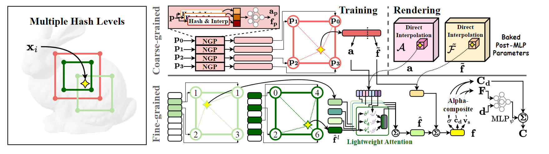
NGP-RT
InstantNGP 虽然训练速度(查询网格)很快,但是渲染的时候仍然需要大量的3D Point查询MLP,耗费大量时间
(Deferred neural rendering) SNeRG [12] 和 MERF [32] 通过将颜色和密度存在显示网格中,只对每条投射光线执行一次 MLP,从而大大加快了渲染过程。然而,他们对显式特征的处理显示出有限的表达能力,不适合 Instant-NGP 的多级特征。将这些特征构建方法直接应用于 Instant-NGP 中的多级特征可能会导致其表示能力受损,并导致渲染质量下降。
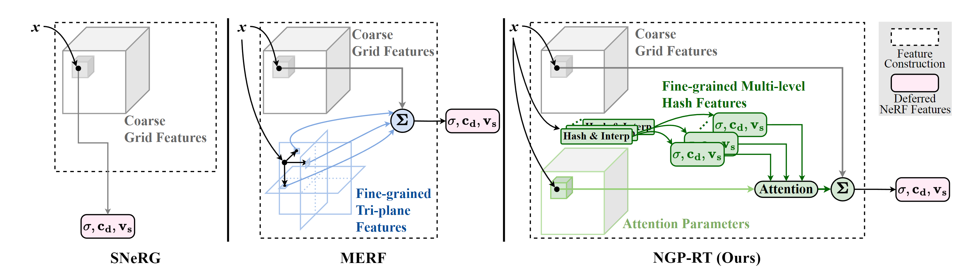
提出了 NGP-RT,一种利用轻量级注意力机制高效渲染高保真新视图的新方法。NGP-RT 的注意力机制采用了简单而有效的加权和运算,可学习的注意力参数可自适应地优先处理显式多级哈希特征
MIMO MLP
Multi input and Multi output MLP(Efficiency of T&R)
(减少MLP计算次数)
MIMO-NeRF
MIMO-NeRF: Fast Neural Rendering with Multi-input Multi-output Neural Radiance Fields
多输入多输出的MLP,同时输入多个三维点来进行计算
Points Sampling
Points Sampling(Efficiency of T&R)
(减少采样点数量 per ray)
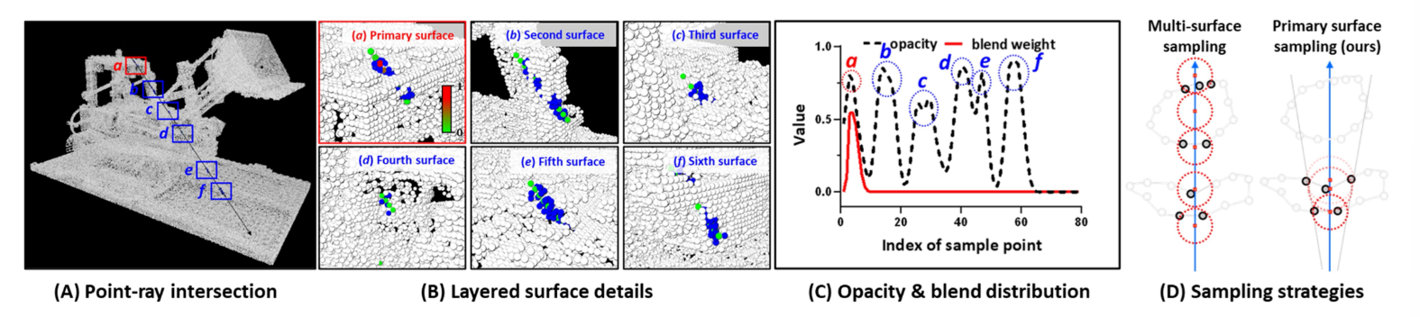
HashPoint
Primary surface point sampling
Pixel Sampling
Pixel Sampling (Efficiency of Training)
(减少MLP计算次数)
之前方法对train_data中所有的像素rgb三个值,进行预测+l1 loss+反向传播,训练速度很慢
通过量化rendering image 与 g.t. image 之间的差异,来指导在图像上采样像素的位置/数量:根据error map between rendering image and g.t. image,消除loss比较小的区域,对loss大的区域进行更多的采样
idea:
- Other sampling method 如果要加速训练的话,就要使用更高效的采样方法
- LHS (Latin hypercube sampling)
- 这种方法只能对Train过程进行加速
- 由于优化的是MLP整体的参数,因此可能出现对误差大的像素优化时,降低误差小的像素的预测精度。
- 可能会对error大但是非重要区域的像素进行多次采样
马尔可夫链蒙特卡罗算法(MCMC) - 知乎 Basic
详解Markov Chain Monte Carlo (MCMC): 从拒绝-接受采样到Gibbs Sampling | Lemon’s Blog 更清楚一点
MCMC详解2——MCMC采样、M-H采样、Gibbs采样(附代码)
采样(三):重要性采样与接受拒绝采样 | Erwin Feng Blog
The Markov-chain Monte Carlo Interactive Gallery 多种MCMC采样方法
Monte Carlo采样无法得到复杂的分布(二维分布),加入Markov Chain,马尔科夫链模型的状态转移矩阵收敛到的稳定概率分布与我们的初始状态概率分布无关$\pi(j)=\sum_{i=0}^\infty\pi(i)P_{ij}$(只与状态转移矩阵有关),如果可以得到状态转移矩阵,就可以采样得到平稳分布的样本集。如何得到状态转移矩阵?
—> MCMC方法(与拒绝-接受采样的思路类似,其通过拒绝-接受概率拟合一个复杂分布, MCMC方法则通过拒绝-接受概率得到一个满足细致平稳条件的转移矩阵.)
- Metropolis-Hastings Sampling:需要计算接受率, 在高维时计算量大, 并且由于接受率的原因导致算法收敛时间变长. 对于高维数据, 往往数据的条件概率分布易得, 而联合概率分布不易得.
- Gibbs Sampling:
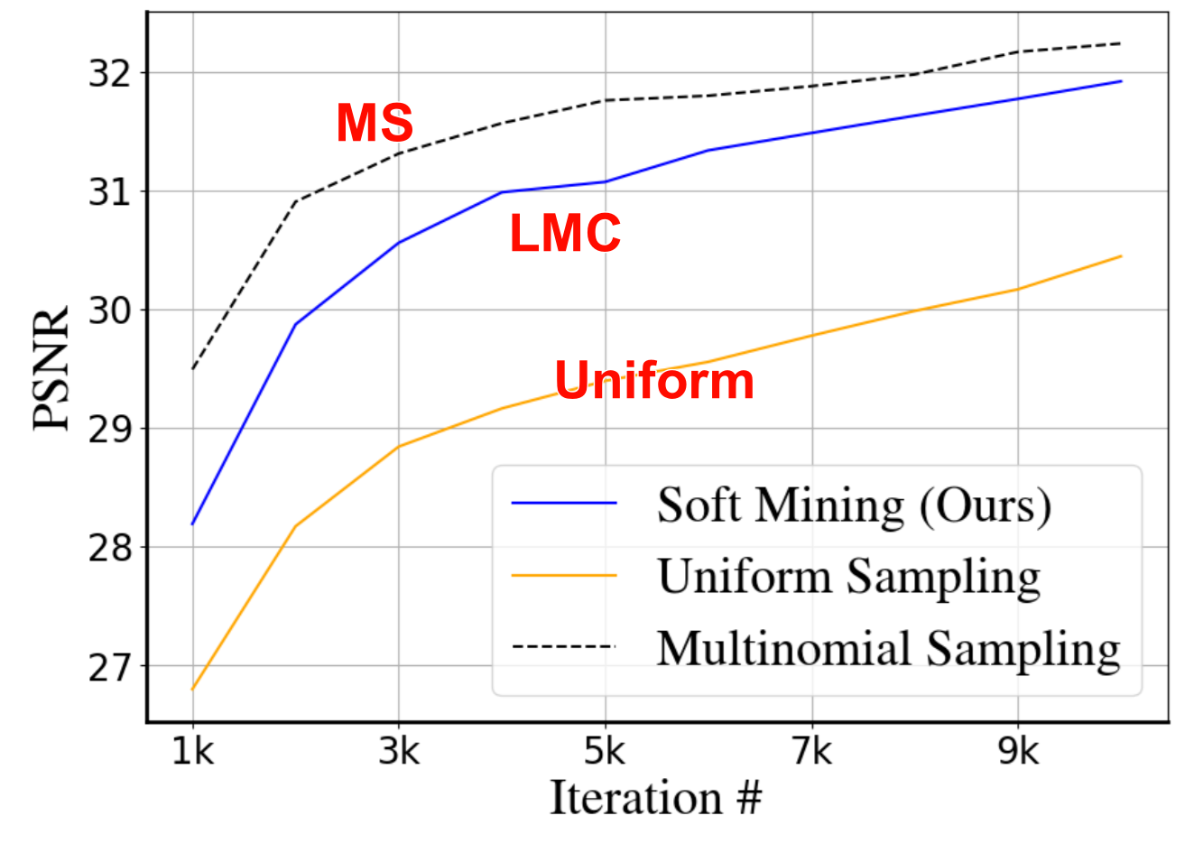
Soft Mining
Accelerating Neural Field Training via Soft Mining
EGRA-NeRF: Edge-Guided Ray Allocation for Neural Radiance Fields NeRF 的渲染显得过于模糊,并且在某些纹理或边缘中包含锯齿伪影,为此提出了边缘引导光线分配(EGRA-NeRF)模块,以在训练阶段将更多光线集中在场景的纹理和边缘上 (没有加速)
To implement our idea we use Langevin Monte-Carlo sampling. We show that by doing so, regions with higher error are being selected more frequently, leading to more than 2x improvement in convergence speed.
$\mathcal{L}=\frac{1}{N}\sum_{n=1}^{N}\mathrm{err}(\mathbf{x}_{n})\approx\mathbb{E}_{\mathbf{x}\sim P(\mathbf{x})}\left[\mathrm{err}(\mathbf{x})\right]=\int\mathrm{err}(\mathbf{x})P(\mathbf{x})d\mathbf{x}$. P is the distribution of the sampled data points $x_{n}$. 之前方法大多是均匀分布
具体做法:
- Soft mining with importance sampling. 引入了 importance distribution$Q(x)$
补充知识 [蒙特卡洛方法] 02 重要性采样(importance sampling)及 python 实现_哔哩哔哩_bilibili 可以从一个任意分布中进行采样
误差可以重写为:$\int\operatorname{err}(\mathbf{x})P(\mathbf{x})d\mathbf{x} =\int\frac{\mathrm{err}(\mathbf{x})P(\mathbf{x})}{Q(\mathbf{x})}Q(\mathbf{x})d\mathbf{x} =\mathbb{E}_{\mathbf{x}\sim Q(\mathbf{x})}\left[\frac{\mathrm{err}(\mathbf{x})P(\mathbf{x})}{Q(\mathbf{x})}\right].$ 由于均匀分布$P(x)$的PDF通常为常数,因此$\mathcal{L}=\frac{1}{N}\sum_{n=1}^{N}\frac{\mathrm{err}(\mathbf{x}_{n})}{Q(\mathbf{x}_{n})}$ $\mathrm{where} \quad\mathbf{x}_{n}\sim Q(\mathbf{x}).$
但是$\mathcal{L}$无法用于训练,采用stop gradient operator(在正向计算时定义为同一值,且偏导数为零)
$\mathcal{L}\approx\mathbb{E}_{\mathbf{x}\sim\mathrm{sg}(Q(\mathbf{x}))}\left[\frac{\mathrm{err}(\mathbf{x})}{\mathrm{sg}(Q(\mathbf{x}))}\right].$
选择的$Q(x)$必须与$err(x)$成比例关系(消除error尺度的影响):$\mathrm{err}(\mathbf{x})=|f_{\boldsymbol{\psi}}(\mathbf{x})-f_{\mathrm{gt}}(\mathbf{x})|_{2}^{2},\\Q(\mathbf{x})=|f_{\boldsymbol{\psi}}(\mathbf{x})-f_{\mathrm{gt}}(\mathbf{x})|_{1}.$
根据$Q(x)$的定义,会在error大的地方多采样一些$x$即像素点
Soft mining. $\mathcal{L}=\frac1N\sum_{n=1}^N\left[\frac{\mathrm{err}(\mathbf{x}_n)}{\mathrm{sg}(Q(\mathbf{x}_n))^\alpha}\right],\quad\text{where }\alpha\in[0,1]$(在关注error大的区域的同时也要关注一下其他区域,不然可能会学歪)
- $\alpha = 0$:hard mining
- $\alpha = 1$:(pure) importance sampling
- Sampling via Langevin Monte Carlo
The promises and pitfalls of Stochastic Gradient Langevin Dynamics 数学分析LMC, SGLD, SGLDFP and SGD
MCMC using Hamiltonian dynamics
从任意分布$Q(x)$中采样,使用MCMC方法中的Langevin Monte Carlo (LMC)
$\mathbf{x}_{t+1}=\mathbf{x}_t+a\nabla\log Q(\mathbf{x}_t)+b\boldsymbol{\eta}_{t+1},$
- a>0 is a hyperparameter defining the step size for the gradient-based walks
- b>0 is a hyperparameter defining the step size for the random walk $\boldsymbol{\eta}_{t\boldsymbol{+}1}\boldsymbol{\sim}\mathcal{N}(0,\mathbf{1})$
- 采样是局部的,因此采样的开销很小
- log的作用应该是把乘除转换成加减, eg: $w_i=\frac{p(x_i)}{q(x_i)}, \log w_i=\log p(x_i)-\log q(x_i)$
Sample (re-)initialization.(采样的初始化很重要):We first initialize the sampling distribution to be uniform over the domain of interest as $\mathbf{x}_{0}{\sim}\mathcal{U}(\mathcal{R})$. We further re-initialize samples that either move out of $\mathcal{R}$ or have too low error value causing samples to get ‘stuck’. We use uniform sampling as well as edge-based sampling for 2D workloads.
Warming up soft mining. Start with $\alpha=0$, i.e., no correction, then linearly increase it to the desired $\alpha$ value at 1k iterations.
Alternative: multinomial sampling. To use multinomial sampling, one needs to do a forward pass of all data points to build a probability density function, which is computationally expensive. Hence an alternative strategy, such as those based on Markov Chain Monte Carlo (MCMC) is required. 为了防止对所有像素点进行前向计算以计算PDF的高耗费,使用MCMC采样
Ablation studies中: 即使LMC采样的精度比multinomial sampling低一点,但仍然比Uniform sampling更高,且更effective(效率与精度的折中(compromise/trade-off))
Shooting Much Fewer Rays
之前的从图片中采样像素or光线的方法:$\mathbf{r}_i(u,v)\sim U(I_i),u\in[0,H_i],v\in[0,W_i],$ 按均匀分布随机采样
- trivial areas:对于背景(大部分颜色相同),这样图片的像素就是非均匀的分布,均匀采样方式会导致采样到一些无意义的像素。 Therefore, we only need to shoot fewer rays in the trivial areas where the color changes slightly to perceive the radiance fields
- nontrivial areas:color changes greatly contain more information, so more rays are required to capture the detailed information and learn how to distinguish these pixels’ colors from its neighboring ones
trivial areas会很快收敛,而nontrivial areas不容易收敛
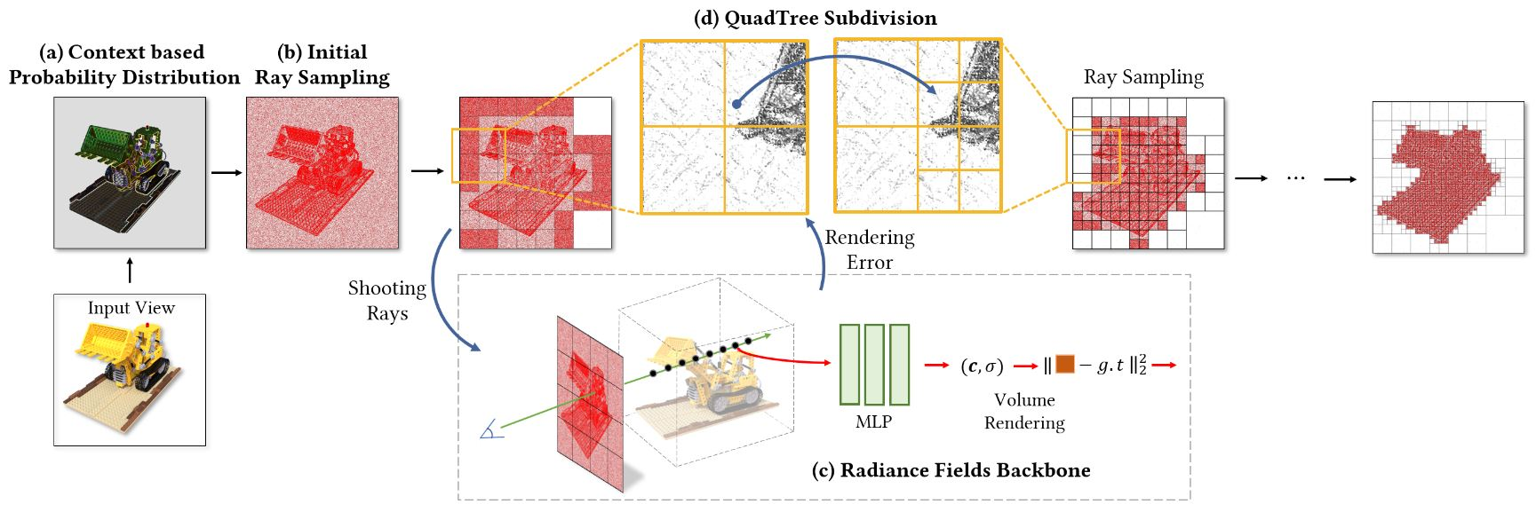
Based on the above observation, we propose two strategies to optimize ray distribution on input images.
- The first one is to calculate a prior probability distribution based on the image context GT图片的先验分布
- the second one is to apply an adaptive quadtree subdivision algorithm to dynamically adjust ray distribution. 自适应的QSA
具体做法:
- Context based Probability Distribution:we use the color variation of pixels relative to their surroundings to quantitatively identify the image context.
计算每个像素点跟周围八个点的std:$g(u,v)=\operatorname{std}(\mathbf{c}(u,v))=\sqrt{\frac19\sum_{x,y}[\mathbf{c}(x,y)-\overline{\mathbf{c}}]^2},\\x\in\{u-1,u,u+1\},y\in\{v-1,v,v+1\}.$ g越高表示像素颜色/密度变化越剧烈,通常在3D物体的表面边界处。优势:our image context based probability distribution function naturally helps to estimate where surfaces are located.
为了平衡$g_{max}$与$g_{min}$之间的差异,clamp后进行归一化:$g^{\prime}(u,v)=\frac{\mathrm{clamp}(s,\max(g(u,v)))}{\mathrm{max}(g(u,v))}$,we typically define threshold $\begin{aligned}s=0.01\times\text{mean}(g(u,v))\end{aligned}$. Values less than s will be clamped to s to avoid sampling too few rays at the corresponding positions.
Sampling strategy. In the lines of “Sampled Rays Distribution”, we sample 50% rays according to the context based probability distribution and randomly sample the other 50% rays, where each red point represents a sampled ray(为什么要设置成50%)
- Adaptive QuadTree Subdivision:对于rendering error,只在error大的地方细分,在error小的地方不在细分(根据pre-defined threshold a来判断大小)
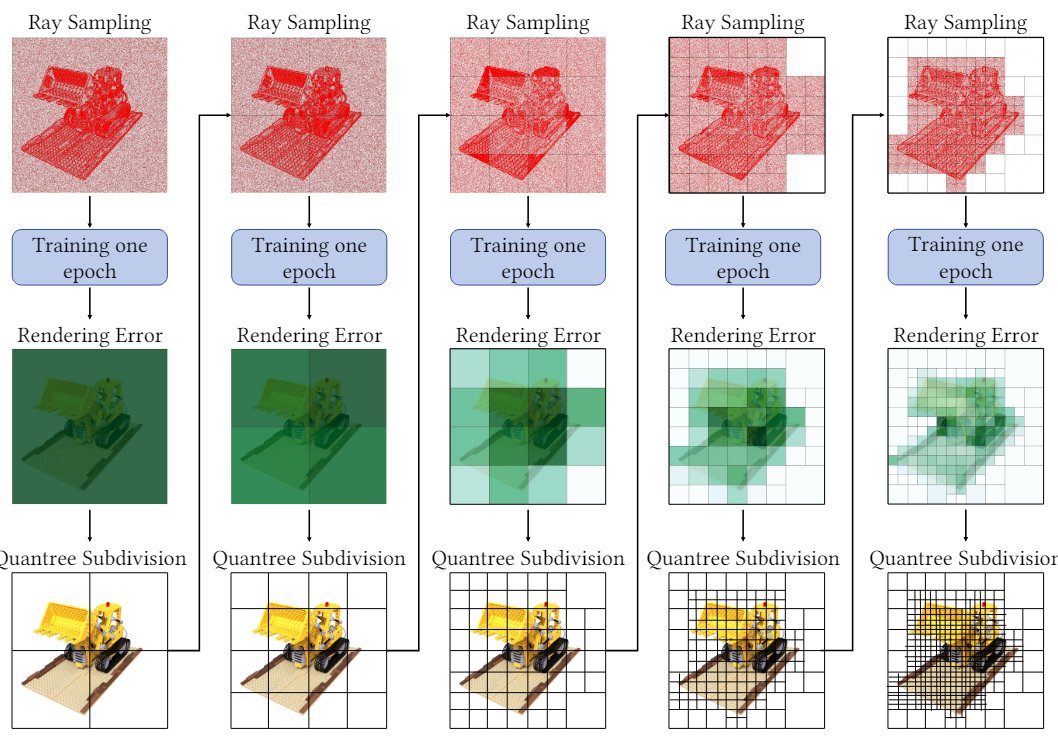
图片$I_{i}(H_{i} \times W_{i})$上总的采样数量:$M_i^l=Q_1^l\times\frac{H_i}{2^l}\times\frac{W_i}{2^l}+Q_2^l\times n_0,$ $l$ denote the times of subdivision, $Q_1^l$ and $Q_2^l$ denote the number of unmarked leaf nodes (error>a) and marked leaf nodes (error<a) separately. $n_{0} = 10(constant)$
同时iMap也使用rendering error来引导采样,不同点:
- The applications of rendering loss are different. iMap uses the rendering loss distribution on image blocks to decide how many points should be sampled on each block, while we use the rendering loss on each leaf node to decide whether this node should be subdivided into 4 child nodes.
- The number of sampled points and image blocks are different. In our method, the number of sampled points in each leaf node is identical, but the number and area of the image blocks (i.e. leaf nodes) changes during training. In contrast, iMap samples different numbers of rays according to a render loss based distribution in each one of the same size blocks.
- The sampling strategies in image blocks are different. In each image block, iMap uniformly samples points for rendering, while we sample points according to the image context. More points are sampled in the nontrivial areas where color changes a lot, while fewer points are sampled in the trivial areas where color changes slightly. Our sampling strategy helps to capture the detailed information in the nontrivial areas and reduce the training burden in the trivial areas.
- Implementation Details
- 在每个epoch结束后,也就是对数据集中所有图像的像素都进行一次rendering,然后与g.t.进行对比得到rendering error
- In practice, we initially subdivide the quadtrees into 2 or 3 depths at the begin of training. This helps our method to distinguish the trivial and nontrivial areas faster among the quadtree leaf nodes
存在的问题:
- All-Pixel Sampling中,作者为了防止MLP对unmarked leaf nodes进行拟合的同时会改变已经拟合好的marked leaf nodes,在接近最后的epoch,使用了randomly sample rays from the whole image instead of using quadtrees for sampling, where the number of sampled rays is equal to the total number of pixels. 如何freeze已经拟合好的marked leaf nodes???
iNeRF
一种基于NeRF预训练模型的姿态估计的方法. 有了NeRF(MLP), 去refine位姿
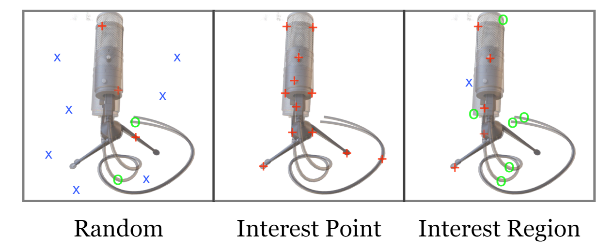
- Sampling Rays: 计算所有pixel是非常耗时耗力的。目的是想要采样的点可以更好的包含在observed images和rendered images上。三种策略:
- Random Sampling
- Interest Point Sampling: employ interest point detectors to localize a set of candidate pixel locations in the observed image, this strategy makes optimization converge faster since less stochasticity is introduced. But we found that it is prone to local minima as it only considers interest points on the observed image instead of interest points from both the observed and rendered images.
- Interest Region Sampling: After the interest point detector localizes the interest points, we apply a 5 × 5 morphological dilation for I iterations to enlarge the sampled region.