MATH
泛函
(72 封私信 / 80 条消息) 「泛函」究竟是什么意思? - 知乎
Calculus of Variations:变分计算 - 分享我的学习心得 变分:自变量x不变,函数$y(\cdot)$改变
研究不同的函数,对输出的影响。
例如MLP要拟合一个函数,让预测的输出与标签非常相近。又如有限元求解偏微分方程,是要根据最小作用量原理,求得一个满足边界条件的、相对准确的近似解
数学基础
摄动法
泰勒
dezeming.top/wp-content/uploads/2021/06/多元函数(及向量函数)的泰勒展开.pdf
泰勒展开本质上是求近似
概率论
Follow:
- 最大似然
- 最大后验
Bayes
贝叶斯定理,改变信念的几何学 - YouTube ——数形结合
走进贝叶斯统计(一)—— 先验分布与后验分布 - 知乎
超详细讲解贝叶斯网络(Bayesian network) - USTC丶ZCC - 博客园
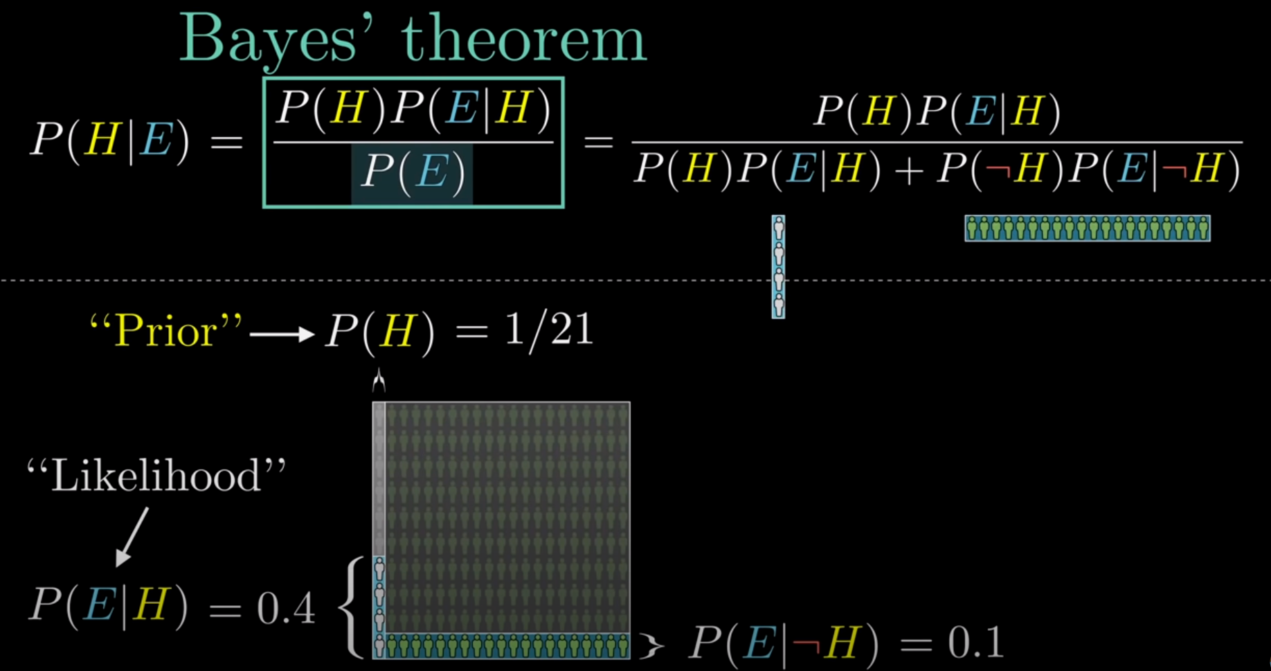
全概率公式:$\mathbf{P(H)}=\mathbf{P(H|A)P(A)}+\mathbf{P(H|B)P(B)}$,结果H发生的概率
贝叶斯公式:$\mathbf{P}(\mathbf{A}|\mathbf{H})=\frac{P(A)P(H|A)}{P(H)}$,H结果发生时,是由A导致的概率
- 连续$p(y_0|x)=\frac{p(x|y_0)p(y_0)}{\int_{-\infty}^{+\infty}p(x|y)p(y)dy}$
- 离散$p(y_j|x)=\frac{p(x|y_j)p(y_j)}{\sum_{i=0}^np(x|y_i)p(y_i)}$
在使用数据估计参数$\theta$之前,我们需要给这个参数设定一个分布,即先验分布$p(\theta)$(根据经验得到)
$p(\theta|X)=\frac{p(\theta,X)}{p(X)}=\frac{p(X|\theta)p(\theta)}{\int_{-\infty}^{+\infty}p(X|\theta)p(\theta)d\theta}.$
- $p(\theta|X)$是$\theta$的后验分布
- $p(X|\theta)$是在给定$\theta$下关于数据样本的似然函数
- $\int_{-\infty}^{+\infty}p(X|\theta)p(\theta)d\theta$ 为常数c,可以写为$p(\theta|X)\propto p(X|\theta)p(\theta).$
Distribution
Gamma Function:$\Gamma(z)=\int_0^\infty t^{z-1}e^{-t}\mathrm{d}t,\quad\Re(z)>0.$ or $\Gamma(n)=(n-1)!.$
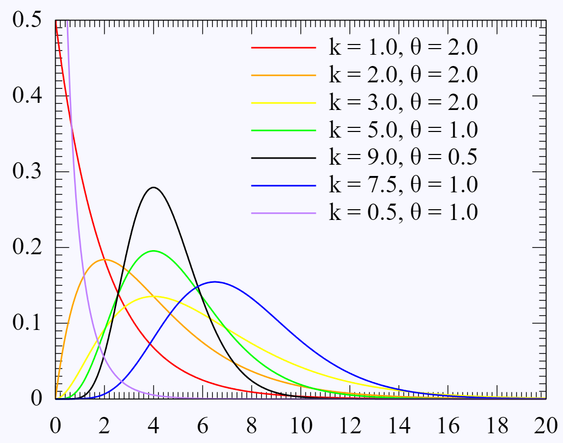
Gamma 分布
$f(x)=\frac{\beta^{\alpha}}{\Gamma(\alpha)}x^{\alpha-1}e^{-\beta x}$
图中k对应$\alpha$,$\theta$对应$\beta$
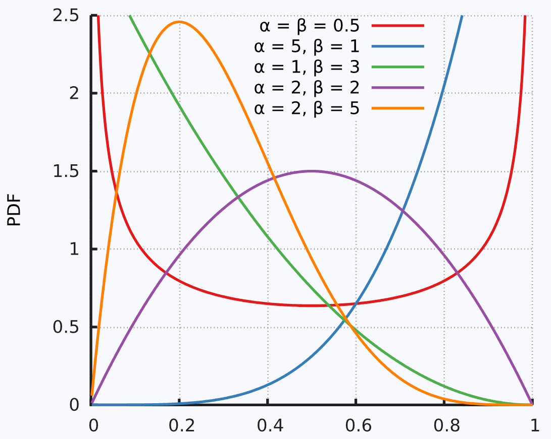
Beta 分布
通常是概率分布的分布
$\mathbf{B}(\alpha,\beta)={\frac{\Gamma(\alpha)\Gamma(\beta)}{\Gamma(\alpha+\beta)}}$
多元高斯分布
多元/多维高斯/正态分布概率密度函数推导 (Derivation of the Multivariate/Multidimensional Normal/Gaussian Density) - 凯鲁嘎吉 - 博客园
多元高斯分布(The Multivariate normal distribution) - bingjianing - 博客园
概率密度函数
$p(x)=p(x_{1},x_{2},\ldots,x_{D})=\frac{1}{(2\pi)^{D/2}}\exp\left(-\frac{1}{2}(x-\mu)^{T}\Sigma^{-1}(x-\mu)\right)$
混合高斯分布
GMM
联合高斯分布
如何构造两个协方差标准分布
AB为两个独立的标准正态分布:
$\begin{aligned}\mathrm{X}&=\alpha\mathrm{A}+\beta\mathrm{B},\\\\\mathrm{Y}&=\gamma\mathrm{A}+\delta\mathrm{B}\end{aligned}$
$\alpha,\beta,\gamma,\delta$是四个待确定的参数,希望找到这四个参数,使得X和Y也服从标准正态分布$N(0,1)$,并且相关系数$Cor(X,Y)=\rho$。
由标准正态分布性质可得:$\mathrm{X}\sim\mathrm{N}(0,\alpha^2+\beta^2),\mathrm{Y}\sim\mathrm{N}(0,\gamma^2+\delta^2)。$
要想:$\bar{\alpha}^{2}+\beta^{2}=1,\gamma^{2}+\delta^{2}=1$
则可以假设:$\alpha=\cos\theta,\beta=\sin\theta;\gamma=\sin\theta,\delta=\cos\theta,$
由相关系数:$\mathrm{Cor(X,~Y)}=\frac{\mathrm{Cov(X,~Y)}}{\sqrt{\mathrm{Var(X)Var(Y)}}}$,$\operatorname{Var}(\mathrm{X})=1$,$\operatorname{Var}(\mathrm{Y})=1$
因此使得:
- ($Cov(A,A)=1,Cov(A,B)=0$)
- $\text{Cov}(x_1 + x_2, y_1 + y_2) = \text{Cov}(x_1, y_1) + \text{Cov}(x_2, y_1) + \text{Cov}(x_1, y_2) + \text{Cov}(x_2, y_2)$
- $\mathrm{Cov}(aX,Y)=a\mathrm{Cov}(X,Y)$
则有:$\theta=\frac{\arcsin\rho}2$,然后令$\begin{cases}\mathrm X=(\cos\theta)\mathrm A+(\sin\theta)\mathrm B\\\mathrm Y=(\sin\theta)\mathrm A+(\cos\theta)\mathrm B\end{cases}$,则计算出来的X和Y就是相关性为$\rho$的标准正态分布
1 | import numpy as np |
P-box
Markov Chains
Sampling
如何在不知道目标概率密度函数的情况下,抽取所需数量的样本,使得这些样本符合目标概率密度函数。这个问题简称为抽样
Finite Element Model Updating in Bridge Structures Using Kriging Model and Latin Hypercube Sampling Method - Wu - 2018 - Advances in Civil Engineering - Wiley Online Library 不同采样方法的讨论(simple random sampling (SRS), stratified sampling method, cluster sampling method, and systematic sampling) Latin Hypercube Sampling 属于 =分层采样
It’s all about Sampling - 子淳的博客 | Just Me
Monte Carlo
一文看懂蒙特卡洛采样方法 - 知乎 (zhihu.com)
简明例析蒙特卡洛(Monte Carlo)抽样方法 - 知乎 (zhihu.com)
走进贝叶斯统计(四)—— 蒙特卡洛方法 - 知乎
逆变换采样和拒绝采样 - barwe - 博客园 (cnblogs.com)
Monte Carlo method - Wikipedia
【数之道 22】巧妙使用”接受-拒绝”方法,玩转复杂分布抽样 - YouTube
MC Sampling
对某一种概率分布p(x)进行蒙特卡洛采样的方法主要分为直接采样、拒绝采样与重要性采样三种:
- Naive Method
- 根据概率分布进行采样。对一个已知概率密度函数与累积概率密度函数的概率分布,我们可以直接从累积分布函数(cdf)进行采样(类似逆变换采样)
- Acceptance-Rejection Method
- 逆变换采样虽然简单有效,但是当累积分布函数或者反函数难求时却难以实施,可使用MC的接受拒绝采样
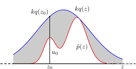
- 对于累积分布函数未知的分布,我们可以采用接受-拒绝采样。如下图所示,p(z)是我们希望采样的分布,q(z)是我们提议的分布(proposal distribution),令kq(z)>p(z),我们首先在kq(z)中按照直接采样的方法采样粒子,接下来判断这个粒子落在途中什么区域,对于落在灰色区域的粒子予以拒绝,落在红线下的粒子接受,最终得到符合p(z)的N个粒子
- 数学推导:
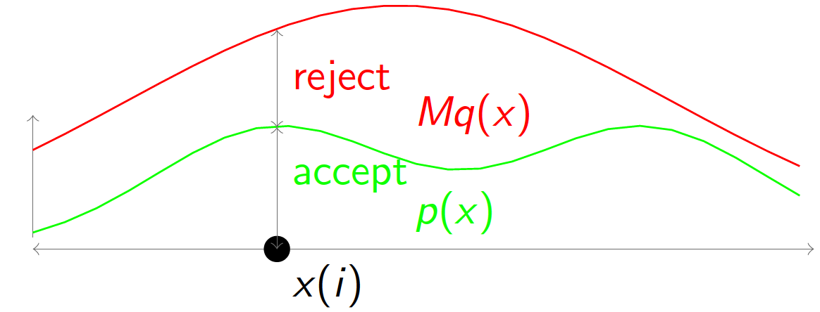
- 从 $f_r(x)$ 进行一次采样 $x_i$
- 计算 $x_i$ 的 接受概率 $\alpha$(Acceptance Probability):$\alpha=\frac{f\left(x_i\right)}{f_r\left(x_i\right)}$
- 从 (0,1) 均匀分布中进行一次采样 u
- 如果 $\alpha$≥u,接受 $x_i$ 作为一个来自 f(x) 的采样;否则,重复第1步
1 | N=1000 #number of samples needed |
- Importance Sampling
- 接受拒绝采样完美的解决了累积分布函数不可求时的采样问题。但是接受拒绝采样非常依赖于提议分布(proposal distribution)的选择,如果提议分布选择的不好,可能采样时间很长却获得很少满足分布的粒子。
- $E_{p(x)}[f(x)]=\int_a^bf(x)\frac{p(x)}{q(x)}q(x)dx=E_{q(x)}[f(x)\frac{p(x)}{q(x)}]$
- 我们从提议分布q(x)中采样大量粒子$x_1,x_2,…,x_n$,每个粒子的权重是 $\frac{p(x_i)}{q(x_i)}$,通过加权平均的方式可以计算出期望:
- $E_{p(x)}[f(x)]=\frac{1}{N}\sum f(x_i)\frac{p(x_i)}{q(x_i)}$
- q提议的分布,p希望的采样分布
1 | N=100000 |
分层采样
分层抖动采样
- 随机采样
- 分层均匀采样
- 分层抖动采样。理想的分层抖动采样很容易陷入维数灾难,因此有人提出了高维转低维采样+随机串联(or随机配对)的方法
Latin Hypercube Sampling
- 将每个维度的区间划分为m个不重叠的区间,每个区间概率相等(取均匀分布,区间大小应相等)
- 从均匀分布中随机采样,每个维度的每个间隔中的一个点
- 将每个维度的点随机配对(相同可能的组合)
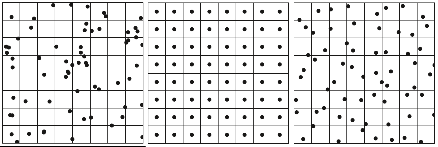
相较于Simple Random Sampling,LHS的方法更加分散,且不存在聚类效应
MCMC
(Markov Chain Monte Carlo)
Blog:
马尔可夫链蒙特卡罗算法(MCMC) - 知乎
动画 The Markov-chain Monte Carlo Interactive Gallery | 代码 Javascript demos
MCMC MCMC: A (very) Beginnner’s Guide
Paper:
An effective introduction to the Markov Chain Monte Carlo method For physics
A Conceptual Introduction to Markov Chain Monte Carlo Methods
Markov Chain Monte Carlo in Practice | W.R. Gilks, S. Richardson, Davi MCMC需要小心地初始化,早期阶段需要warm-up time
M-H采样
Gibbs采样
TMCMC
拉丁超立方采样(Latin hypercube sampling, LHS)
拉丁超立方采样先把样本空间分层,在此问题下要分为5层,于是便有了 [1,20],[21,40],[41,60],[61,80],[81,100] 共5个样本空间,在各样本空间内进行随机抽样,然后再打乱顺序,得到结果。这样就结束了~
可以看出拉丁超立方采样分为了三步——分层、采样、乱序。
Langevin Monte Carlo(LMC)
Hamiltonian Monte Carlo(HMC)
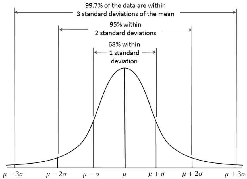
置信区间
图像展示
箱型图
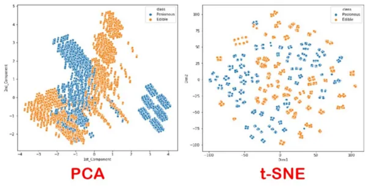
t-SNE 数据降维
降维方法之t-SNE - 知乎
Everything About t-SNE. t-SNE means t-distribution Stochastic… | by Ram Thiagu | The Startup | Medium
PCA是一种常用的降维方式,但是不方便展示结果。例如对两类数据进行降维(二维),PCA和t-SNE两种方法的展示结果为:
线性代数
特殊矩阵定义
正交矩阵 正交矩阵 - 维基百科,自由的百科全书
- $Q^T=Q^{-1}\Leftrightarrow Q^TQ=QQ^T=I.$ 其中$I$为单位矩阵
- 正交矩阵的行列式值必定为+1或−1。
- 行列式值为+1的正交矩阵,称为特殊正交矩阵,它是一个旋转矩阵。
- 行列式值为-1的正交矩阵,称为瑕旋转矩阵。瑕旋转是旋转加上镜射。镜射也是一种瑕旋转。
正定矩阵【线性代数】详解正定矩阵、实对称矩阵、矩阵特征值分解、矩阵 SVD 分解 - 知乎
- 任意非零向量$\mathbf{x}$,若$\mathbf{x}^{T}\mathbf{A}\mathbf{x}>0$恒成立,则$\mathbf{A}$为正定矩阵。若$\mathbf{x}^{T}\mathbf{A}\mathbf{x}\geq0$恒成立,则$\mathbf{A}$为半正定矩阵
变换
2D
仿射变换
3D
像素Pixel | 相机Camera | 世界World
内参矩阵 = c2p
外参矩阵 = w2c
根据世界坐标计算像素坐标 = c2p * w2c * world_position
Computer Graphics
SDF计算与求导
空间中的子集$\partial\Omega$,SDF值定义为:$\left.f(x)=\left\{\begin{array}{ll}d(x,\partial\Omega)&\mathrm{~if~}x\in\Omega\-d(x,\partial\Omega)&\mathrm{~if~}x\in\Omega^c\end{array}\right.\right.$
其中$d(x,\partial\Omega):=\inf_{y\in\partial\Omega}d(x,y)$表示x到表面子集上一点的距离,inf表示infimum最大下界
Computer Vision
卷积图像大小计算公式
图像卷积后的大小计算公式: $N=\left\lfloor\frac{W-F+2P}{Step}\right\rfloor+1$
- 输入图片大小 $W \times W$
- Filter(卷积核)大小 $F \times F$
- 步长 Step
- padding(填充)的像素数 $P$
- 输出图片的大小为$N \times N$
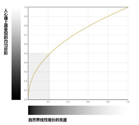
linearColor 2 sRGB
(Why)为什么要将线性RGB转换成sRGB
小tip: 了解LinearRGB和sRGB以及使用JS相互转换 « 张鑫旭-鑫空间-鑫生活 (zhangxinxu.com)
人这种动物,对于真实世界的颜色感受,并不是线性的,而是曲线的
(How)线性RGB与sRGB相互转化
1 | def linear_to_srgb(linear): |
Other
数据处理方法
SOM(自组织映射神经网络)——理论篇 - 知乎
自组织映射(SOM)理论基础与Python NumPy实现 | 美美智能博客站
针对数据量大的情况
自组织映射(Self-organizing map, SOM)通过学习输入空间中的数据,生成一个低维、离散的映射(Map),从某种程度上也可看成一种降维算法。(降维或者升为可以由输入和输出尺寸决定,SOM输入为1E6,输出为70x70,本质上数据量变少,因此为降维算法)
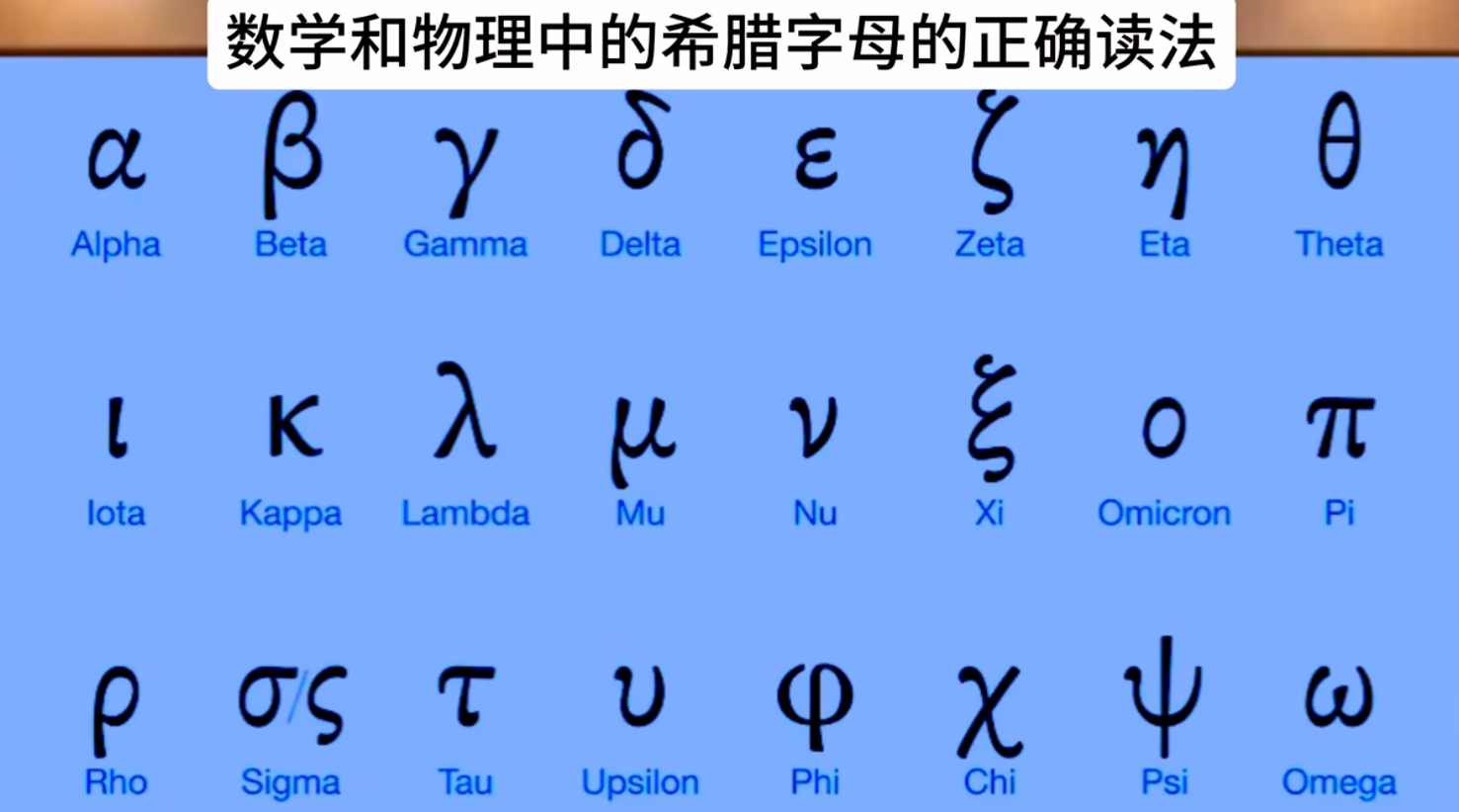
希腊字母