Loss Functions and Metrics in Deep Learning 这篇Review中提到的loss函数比较全面

Loss Functions vs. Performance Metrics
损失函数在训练过程中用于优化模型参数。它衡量的是模型预测输出与预期输出之间的差值，而训练的目标就是尽量减小这一差值。(可微)
性能指标用于评估训练后的模型。它衡量的是模型对新数据的泛化程度以及预测的准确性。性能指标还可以对不同的模型或配置进行比较，以确定性能最佳的模型或配置。(不需要可微)

常用的loss

L1 Loss(MAE, Mean Absolute Error)

$MAE =\sum_{i=1}^n|y_i-\hat{y_{i}}|$

$y_i$为真实值
$\hat{y_{i}}$为预测值

L2 Loss(MSE, Mean Squared Error)

$MSE=\sum_{i=1}^n(y_i-\hat{y_{i}})^2$

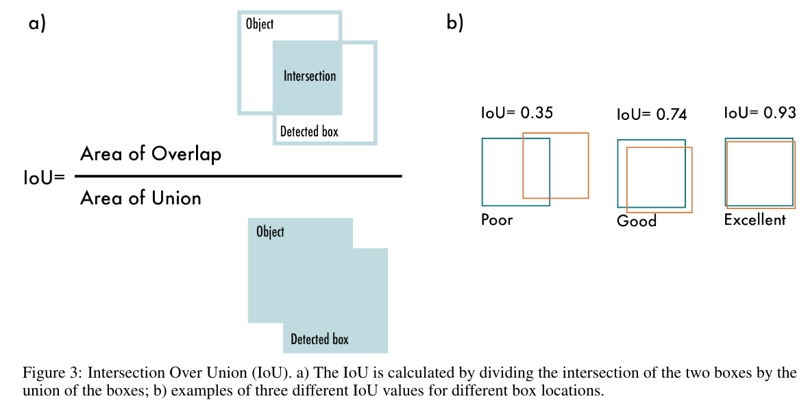
交并比损失(IoU, Intersection over Union)

$IoU=\frac1n\sum_{i=1}^n\frac{y_i\cap\hat{y_i}}{y_i\cup\hat{y_i}}$

交叉熵损失(Cross Entropy Loss)

损失函数｜交叉熵损失函数

二分类(BCE, Binary Cross-Entropy Loss)

$L=\frac{1}{N}\sum_{i}L_{i}=\frac{1}{N}\sum_{i}-[y_{i}\cdot log(p_{i})+(1-y_{i})\cdot log(1-p_{i})]$

$y_i$表示样本$i$的label，正类为1，负类为0
$p_i$样本$i$预测为正类的概率

多分类(CCE, Categorical Cross-entropy Loss)

$L=\frac{1}{N}\sum_iL_i=-\frac{1}{N}\sum_i\sum_{c=1}^My_{ic}\log(p_{ic})$

Time series Loss

FFT Loss

(Fast fourier transform and convolution algorithms)

DIFFUSION-TS: INTERPRETABLE DIFFUSION FOR GENERAL TIME SERIES GENERATION

# target: batch_size, seq_length, feature_dim
# loss_fn is L1 loss or L2 loss

train_loss = self.loss_fn(model_out, target, reduction='none')

fft1 = torch.fft.fft(model_out.transpose(1, 2), norm='forward')
fft2 = torch.fft.fft(target.transpose(1, 2), norm='forward')

fft1, fft2 = fft1.transpose(1, 2), fft2.transpose(1, 2)
fourier_loss = self.loss_fn(torch.real(fft1), torch.real(fft2), reduction='none')\
               + self.loss_fn(torch.imag(fft1), torch.imag(fft2), reduction='none')
train_loss +=  self.ff_weight * fourier_loss

三维重建 Loss Functions

Eikonal loss

Implicit Geometric Regularization for Learning Shapes

确保SDF在空间中的梯度大小保持恒定，这有助于保持SDF场的一致性和准确性

$\mathcal{L}_{r e g}=\frac{1}{n m}\sum_{k,i}(\|\nabla f(\hat{\mathbf{p}}_{k,i})\|_{2}-1)^{2}.$

RGB Loss

L2 损失：F.mse_loss(pred_rgb, gt_rgb) $L=\sum_{i=1}^n(y_i-f(x_i))^2$
L1 损失：F.l1_loss(pred_rgb, gt_rgb)更稳定？ $L=\sum_{i=1}^n|y_i-f(x_i)|$

Mask Loss

$\mathcal{L}_{mask}=\mathrm{BCE}(M_k,\hat{O}_k)$

$\hat{O}_k=\sum_{i=1}^n T_{k,i}\alpha_{k,i}$
$M_{k} ∈ {0, 1}$

BCE 二值交叉熵损失：让输出$\hat{O}_k$去逼近 label $M_{k}$

Spatial-BCE

一种新的 BCE lossECCV’22 ｜ Spatial-BCE - 知乎 (zhihu.com)

Opacity Loss

loss_opaque = -(opacity * torch.log(opacity) + (1 - opacity) * torch.log(1 - opacity)).mean()
$opaque = BCE(opaque,opaque) = -[opaque ln(opaque) + (1-opaque) ln(1-opaque)]$

使得 opacity 更加接近 0 或者 1

Sparsity Loss

loss_sparsity = torch.exp(-self.conf.loss.sparsity_scale * out['sdf_samples'].abs()).mean()
$sparsity = \frac{1}{N} \sum e^{-scale * sdf}$
让 sdf 的平均值更小，前景物体更加稀疏，物体内的点往外发散

Geo-Neus

sdf loss
- sdf_loss = F.l1_loss(pts2sdf, torch.zeros_like(pts2sdf), reduction='sum') / pts2sdf.shape[0]
- $\mathcal{L}_{sdf} = \frac{1}{N} \sum |sdf(spoint) - 0|$

Other loss

加强Eikonal对SDF的优化

sunyx523/StEik (github.com)
NeurIPS 2023 | 三维重建中的Neural SDF(Neural Implicit Surface) - 知乎 (zhihu.com)
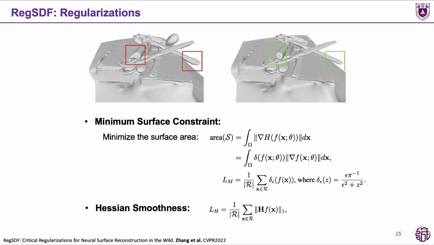
一个好的SDF其实只需要其法线方向上的二阶导数为0，如果在切线方向上的二阶导数为0的话，得到的SDF轮廓会非常平滑，不利于学习到一些细节。

$L_\text{L. n.}(u)=\int_{\Omega}|\nabla u(x)^TD^2u(x)\cdot\nabla u(x)|dx.$

随机结构相似性损失(S3IM, Stochastic Structural SIMilarity loss)

Project Page S3IM Stochastic Structural SIMilarity and Its Unreasonable Effectiveness for Neural Fields
Paper S3IM: Stochastic Structural SIMilarity and Its Unreasonable Effectiveness for Neural Fields

$\begin{aligned}L_{\mathrm{S3IM}}(\Theta,\mathcal{R})=&1-\mathrm{S3IM}(\hat{\mathcal{R}},\mathcal{R})\\=&1-\frac1M\sum_{m=1}^M\mathrm{SSIM}(\mathcal{P}^{(m)}(\hat{\mathcal{C}}),\mathcal{P}^{(m)}(\mathcal{C})).\end{aligned}$

Smoothness Loss

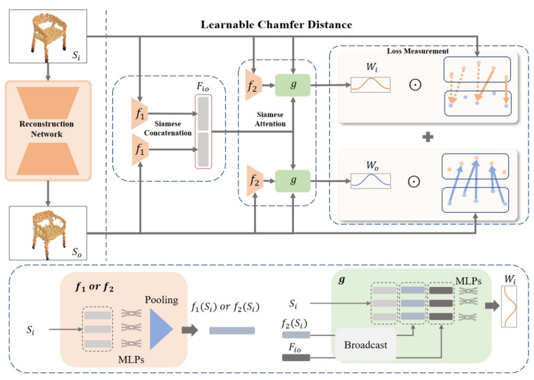
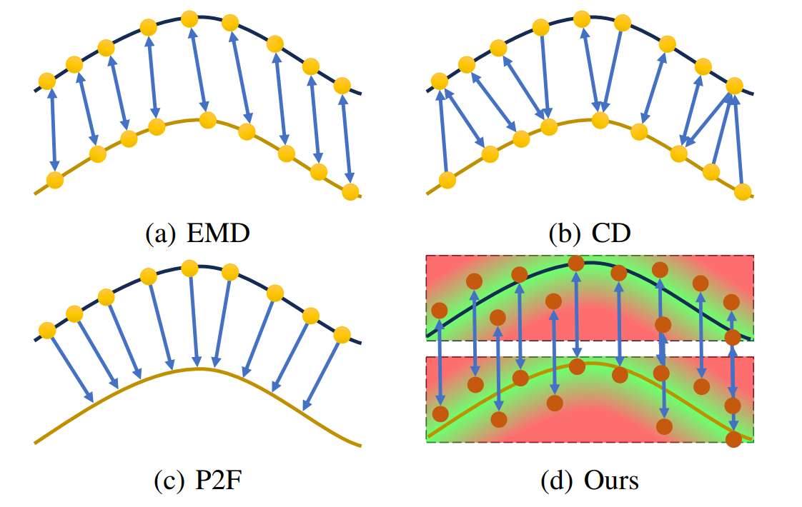
可学习倒角距离(LCN, Learnable Chamfer Distance)

Learnable Chamfer Distance for Point Cloud Reconstruction

$\begin{aligned}L_{R}(S_{i},S_{o})&=\frac12(\frac1{|S_i|}\sum_{x\in S_i}W_i\cdot\min_{y\in S_o}\|x-y\|_2\\&+\frac1{|S_o|}\sum_{x\in S_o}W_o\cdot\min_{y\in S_i}\|x-y\|_2).\end{aligned}$

我们提出了一种简单但有效的重建损失，称为可学习倒角距离（LCD），通过动态关注由一组可学习网络控制的不同权重分布的匹配距离

DirDist

[2401.09736] Measuring the Discrepancy between 3D Geometric Models using Directional Distance Fields (arxiv.org)

三维重建 Performance Metrics

倒角距离(CD↓, Chamfer Distance)

jzhangbs/DTUeval-python: A fast python implementation of DTU MVS 2014 evaluation (github.com)

点云或 mesh 重建模型评估指标，它度量两个点集之间的距离，其中一个点集是参考点集，另一个点集是待评估点集

$d_{\mathrm{CD}}(S_1,S_2)=\frac{1}{S_1}\sum_{x\in S_1}\min_{y\in S_2}\lVert x-y\rVert_2^2+\frac{1}{S_2}\sum_{y\in S_2}\min_{x\in S_1}\lVert y-x\rVert_2^2$

$S_{1}$ 和 $S_{2}$ 分别表示两组 3D 点云，第一项代表 $S_{1}$ 中任意一点 x 到 $S_{2}$ 的最小距离之和，第二项则表示 $S_{2}$ 中任意一点 y 到 $S_{1}$ 的最小距离之和。

如果该距离较大，则说明两组点云区别较大；如果距离较小，则说明重建效果较好。

$\begin{aligned}\mathcal{L}_{CD}&=\sum_{y’\in Y’}min_{y\in Y}||y’-y||_2^2+\sum_{y\in Y}min_{y’\in Y’}||y-y’||_2^2,\end{aligned}$

PSNR↑

峰值信噪比 Peak Signal to Noise Ratio
PSNR 是一个无参考的质量评估指标
$PSNR(I)=10\cdot\log_{10}(\dfrac{MAX(I)^2}{MSE(I)})$
$MSE=\frac1{mn}\sum_{i=0}^{m-1}\sum_{j=0}^{n-1}[I(i,j)-K(i,j)]^2$
$MAX(I)^{2}$（动态范围可能的最大像素值，b 位：$2^{b}-1$），eg: 8 位图像则$MAX(I)^{2} = 255$

# Neus
psnr = 20.0 * torch.log10(1.0 / (((color_fine - true_rgb)**2 * mask).sum() / (mask_sum * 3.0)).sqrt())

# instant-nsr-pl
psnr = -10. * torch.log10(torch.mean((pred_rgb.to(gt_rgb)-gt_rgb)**2))

SSIM↑

VainF/pytorch-msssim: Fast and differentiable MS-SSIM and SSIM for pytorch. (github.com)

结构相似性 Structural Similarity Index Measure
SSIM 是一个完整的参考质量评估指标。
$SSIM(x,y)=\dfrac{(2\mu_x\mu_y+C_1)(2\sigma_{xy}+C_2)}{(\mu_x^2+\mu_y^2+C_1)(\sigma_x^2+\sigma_y^2+C_2)}$
衡量了两张图片之间相似度：($C_1,C_2$为常数防止除以 0)

$S(x,y)=l(x,y)^{\alpha}\cdot c(x,y)^{\beta}\cdot s(x,y)^{\gamma}$

$C_1=(K_1L)^2,C_2=(K_2L)^2,C_3=C_2/2$
$K_{1}= 0.01 , K_{2} = 0.03 , L = 2^{b}-1$

亮度，图像 x 与图像 y 亮度 $l(x,y) =\frac{2\mu_x\mu_y+C_1}{\mu_x^2+\mu_y^2+C_1}$
- $\mu_{x} =\frac1N\sum_{i=1}^Nx_i$像素均值
  - $x_i$像素值，N 总像素数
- 当 x 与 y 相同时，$l(x,y) = 1$
对比度，$c(x,y)=\frac{2\sigma_x\sigma_y+C_2}{\sigma_x^2+\sigma_y^2+C_2}$
- 图像标准差$\sigma_x=(\frac1{N-1}\sum_{i=1}^N(x_i-\mu_x)^2)^{\frac12}$
结构对比，$s(x,y)=\frac{\sigma_{xy}+C_3}{\sigma_x\sigma_y+C_3}$ - 图像的协方差$\sigma_{xy}=\frac1{N-1}\sum_{i=1}^N(x_i-\mu_x)(y_i-\mu_y)$
实际使用中(圆对称高斯加权公式)，使用一个高斯核对局部像素求 SSIM，最后对所有的局部 SSIM 求平均得到 MSSIM

使用高斯核，均值、标准差和协方差变为：
$\mu_{x}=\sum_{i}w_{i}x_{i}$
$\sigma_{x}=(\sum_{i}w_{i}(x_{i}-\mu_{x})^{2})^{1/2}$
$\sigma_{xy}=\sum_{i}w_{i}(x_{i}-\mu_{x})(y_{i}-\mu_{y})$

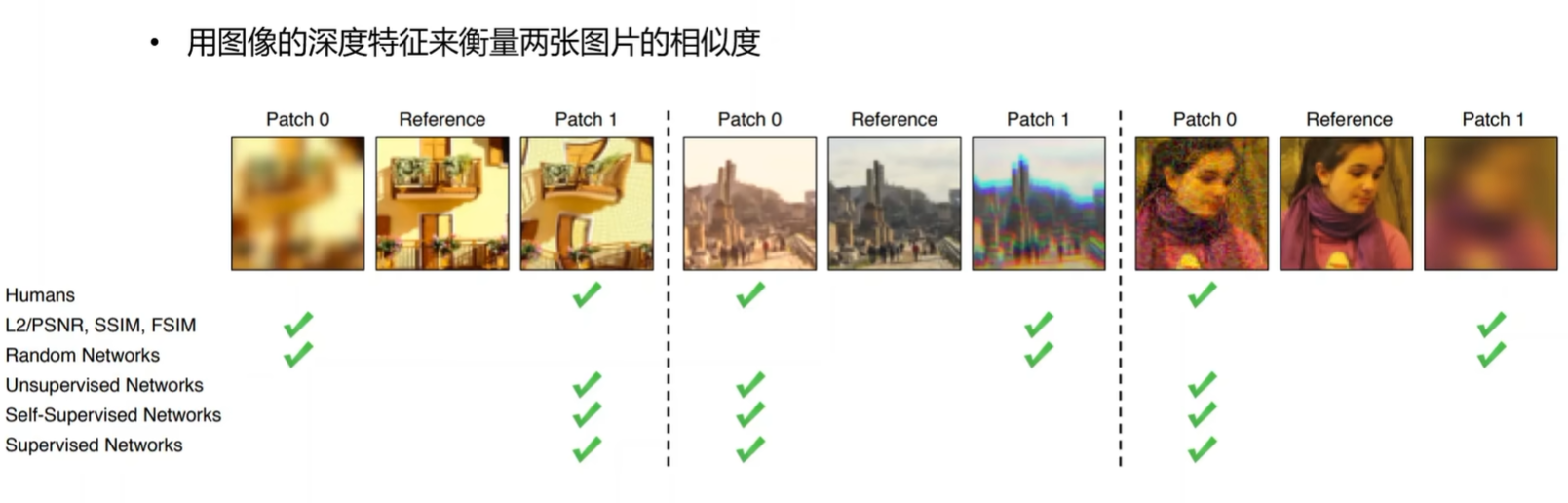
学习感知图像块相似度(LPIPS↓, Learned Perceptual Image Patch Similarity)

The Unreasonable Effectiveness of Deep Features as a Perceptual Metric

LPIPS 比传统方法（比如 L2/PSNR, SSIM, FSIM）更符合人类的感知情况。LPIPS 的值越低表示两张图像越相似，反之，则差异越大。。LPIPS 是一个完整的参考质量评估指标，它使用了学习的卷积特征。分数是由多层特征映射的加权像素级 MSE 给出的。

$LPIPS(x,y)=\sum\limits_{l}^{L}\dfrac{1}{H_lW_l}\sum\limits_{h,w}^{H_l,W_l}||w_l\odot(x^l_{hw}-y^l_{hw})||^2_2$

平均点到面距离(P2S↓, average point-to-surface distance)

ICON: Implicit Clothed humans Obtained from Normals

P2S距离： 是CD的单向版本。(CAPE数据集scan包含大的空洞，为了排除孔洞影响，ICON论文记录scan点到最近重构表面点之间距离)

Normal↓

average surface normal error平均表面法向损失

Normal difference: 表示使用重构的及真值surface分别进行渲染normal图片，计算两者之间L2距离，用于捕获高频几何细节误差。
For both reconstructed and ground truth surfaces, we render their normal maps in the image space from the input viewpoint respectively. We then calculate the L2 error between these two normal maps.

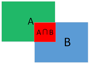
IoU↑

Intersection over Union(IoU)交并比
在目标检测中用到的指标$IOU = \frac{A \cap B}{A \cup B}$
一般来说，这个比值＞ 0.5 就可以认为是一个不错的结果了。

A: GT bounding box
B: Predicted bounding box

推土距离(EMD↓, Earth Mover’s distance)

[2102.12833] Diffusion Earth Mover’s Distance and Distribution Embeddings
EMD(earth mover’s distances)距离 - 知乎 (zhihu.com)
Earth Mover’s Distance (EMD) loss · Issue #211 · facebookresearch/pytorch3d
EMD指标可以用来评价结果，但是无法用作损失loss，已有的loss_ED无法用于中型规模以上的点云中

度量两个分布之间的距离，$\phi$ indicates a parameter of bijection.

$d_{EMD}(S_1,S_2)=\min_{\phi:S_1\to S_2}\sum_{x\in S_1}\|x-\phi(x)\|_2$

$\mathcal{L}_{EMD}=min_{\phi:Y\rightarrow Y^{\prime}}\sum_{x\in Y}||x-\phi(x)||_{2}$ , φ indicates a parameter of bijection.

Accuracy、Precision、Recall & F-score

如何解释召回率与精确率？ - 朝暾的回答 - 知乎
 机器学习的评价指标（一）：Accuracy、Precision、Recall、F1 Score - 知乎 (zhihu.com)

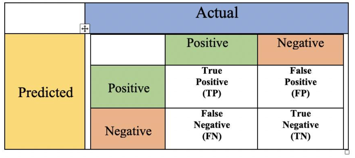
Accuracy

预测正确的样本数÷样本数总数
$accuracy=\frac{TP+TN}{TP+TN+FP+FN}$

Precision

精确率是针对我们预测结果而言的，它表示的是预测为正的样本中有多少是真正的正样本。
$precision=\frac{TP}{TP+FP}$

Recall

召回率是针对我们原来的样本而言的，它表示的是原来样本中的正例有多少被预测正确了，也即真实准确的正预测在原来样本的正例中所占的百分比。
$recall=sensitivity=\frac{TP}{TP+FN}$

F-score

F-Measure是Precision和Recall的加权调和平均
$F=\frac{(a^2+1)precisionrecall}{a^2*precision+recall}$

当参数α=1时，就是最常见的F1，也即$F1=\frac{2precisionrecall}{precision+recall}$